
3D FEM S IMULATION AND O PTIMIZATION F RAMEWORK FOR C OMPUTATIONAL E LECTROMAGNETICS
Users Guide
©2024 EM I NVENT SP. Z O. O. (LTD.)
T RZY L IPY 3 , 80-172 G DANSK , P OLAND
www.inventsim.com
Contents
1 Overview
InventSim is a 3D simulation and design optimization framework for accurate and efficient solutions for various electromagnetic problems arising in the design of complex, high frequency circuits.
The package consists of a 3D geometry modeler, a 3D FEM solver and a set of tools for postprocessing the simulation results. The solver used in InventSim is a general 3D finite element package for solving closed or open domain electromagnetic problems arising in the analysis of microwave junctions, filters, couplers, multiplexers or antennas. From its origins, the software was targeting the design of high frequency, microwave and terahertz passive electronic components, but nowadays it can also be applied in solving problems arising in other fields, like photonics.
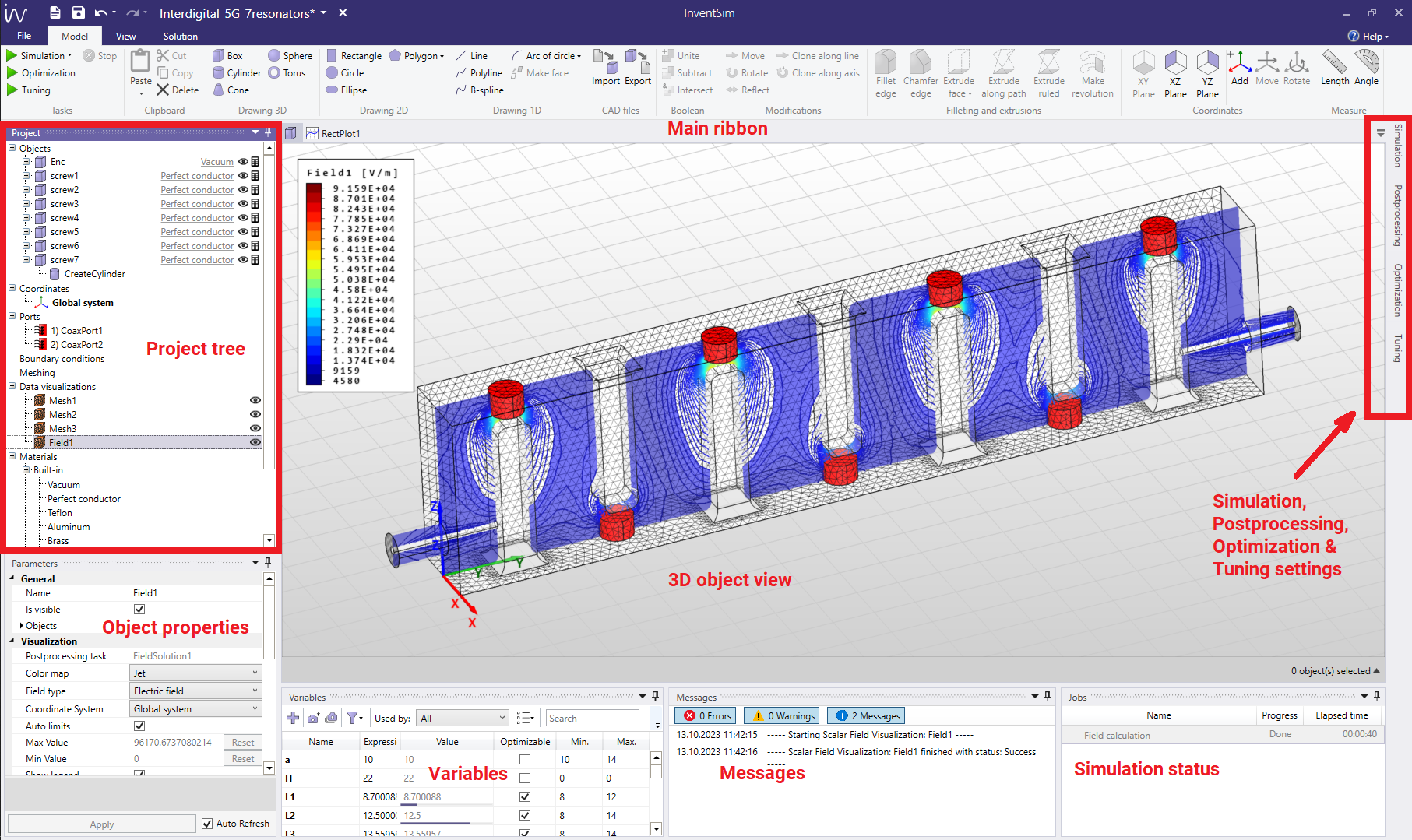
The graphical user interface of InventSim consists of few major parts:
-
• 3D view.
-
• Ribbon with tools (toolbar).
-
• Project tree.
-
• Object parameters panel.
-
• Simulation settings panel.
-
• Messages and simulation status panels.
as seen in the Fig. 1.1, the 3D view uses DirectX API to draw three-dimensional objects onto the screen. The 3D view allows you to:
-
• Create objects by drawing them.
-
• Manipulate existing objects via a mouse.
-
• Visualize additional data.
The toolbar in the upper part of the window allows a quick access to most of the modeler functions: performing operations on objects, adding and modifying coordinate systems, etc. The project panel is a tree panel, grouping and visualizing all project data such as structures (SimObjects), variables and coordinate system. Opject parameters’ panel displays parameters of currently selected objects/items.
The finite element method applied for Maxwell’s equations is one of the computational electromagnetic techniques that allows you to solve boundary-value problems [1, 2, 3, 4] for complex, user-defined structures which finds application in many fields of science. The standard finite element problem defined in InventSim is to solve the electric field vector wave equation
\(\seteqnumber{0}{}{0}\)\begin{equation} \label {helm} \nabla \times \mu ^{-1} \nabla \times \emph {\textbf {E}} - \omega ^2 \epsilon \emph {\textbf {E}} = 0 \end{equation}
in the frequency domain with suitable, user-defined boundary conditions. Applying Galerkin’s method to the wave equation gets you a fundamental FEM equation (called weak form equation)
\(\seteqnumber{0}{}{1}\)\begin{equation} \label {helm2} \int _V \emph {\textbf {W}} \cdot \left ( \nabla \times \mu ^{-1} \nabla \times \emph {\textbf {E}} - {k_0}^2 \epsilon _r \emph {\textbf {E}} \right ) dV = 0 \end{equation}
InventSim allows you to solve the equation (2) with field represented with a set of vector basis functions \(\emph {\textbf {W}}\) up to the third order (QT\(\backslash \)CuN - quadratic tangential and cubic normal) and curvilinear tetrahedral elements (second order unstructured mesh) [8, 10, 11]. To compute the transfer function, an approach presented in [9] is used.
1.1 Main features
3D Modeler main features list:
-
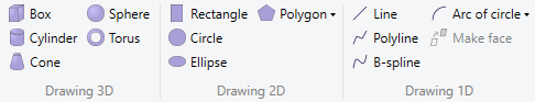
• Draw basic 3D and 2D objects using predefined basic shapes: box, cylinder, cone, sphere, torus, rectangle, circle, ellipse,
-
• Perform Boolean operations on objects: unite, subtract, intersect,
-
• Move, rotate, clone objects,
-
• Fillet of chamfer edge of an object,
-
• Extrude 2D objects,
-
• Define variables and equations,
-
• Define nested coordinate systems,
-
• Import/export of external 3D solids with .STEP file format.
3D FEM solver main features list:
-
• High order basis functions for accurate approximation of electromagnetic fields,
-
• Second order curvilinear tetrahedral elements for accurate modeling of curved geometries,
-
• Arbitrary shaped ports with TEM, TE/TM and hybrid modes,
-
• Handling of both lossy dielectric and conductor materials,
-
• Advanced fast frequency sweep algorithms,
-
• Antenna simulation including absorbing boundary conditions,
-
• Near-To-Far field transformation for open problems (radiation),
-
• Handling complex materials, such as gyromagnetic or Debye dielectrics.
EM Invent is based on industry-proven, highly-accurate higher order finite elements on curvilinear tetrahedral mesh. It takes advantage of these unique technologies:
-
• QuickTune and OptiFast: two techniques that speed up design and optimization. While OptiFast is used for automated optimization, QuickTune is used for iterative design tuning based on full wave computations.
-
• Stretchable-mesh: eliminates the response noise and allows EM Invent to bypass the time-consuming re-meshing every time the structure dimensions change. (elastic or deformable mesh)
-
• ZPO: zero-pole optimization that allows for fast and (often) automated design of pseudoelliptic microwave filters and optimization of their passband performance
-
• Interoperability with other apps using built-in Component Object Model (COM) interface.
1.2 Requirements and Installation
InventSim software is targeted for 64bit (x64) versions of Microsoft Windows OS. The installation requires administrative privileges. The software installation package comes with the main installer application: "EM_Invent_Simulator _Installer.exe". The prerequisites are installed automatically, if needed, by the main installer.
The software requirements of the simulator are:
-
1. 64-bit Windows operating system (including all updates),
-
2. .NET 4.5 Framework,
-
3. Sentinel HASP run-time environment (for Full version only)
-
4. Visual C++ run-time libraries.
The hardware requirements are:
-
1. 64-bit processor with AVX2 support,
-
2. 8GB of RAM memory,
-
3. at least 600MB of disk space.
The electromagnetic simulation procedure is a memory intensive process: a minimum of 16GB RAM memory is recommended for solution of small problems, while electrically large, complex circuits might demand hundreds of gigabytes of RAM ( 512GB). The RAM requirements are therefore problem-dependent.
In order to use the Full version of InventSim (see EULA at the end of this document) you should install the Thales Sentinel HASP Hardware Key drivers (bundled in the installation package) and have the valid hardware license key from EM Invent.
2 Quckstart: Simulation of a microstrip stub
Let us begin with the task of simulating a electromagnetic field and a transfer function for a device that consists of a stub that is connected in parallel to planar transmission line printed on the dielectric layer. This type of structure is called a microstrip line with a stub in microwave engineering.
In most cases, the electromagnetic field simulation of any device (or circuit) with InventSim would consist of three basic steps:
-
1. Definition of geometry of the structure, materials and the boundary conditions,
-
2. Setting the simulation options (meshing, frequency plan, solution technique),
-
3. Visualization of simulation results (electromagnetic field distribution and/or transfer function).
2.1 Construction of a 3D model
To create a 3D model:
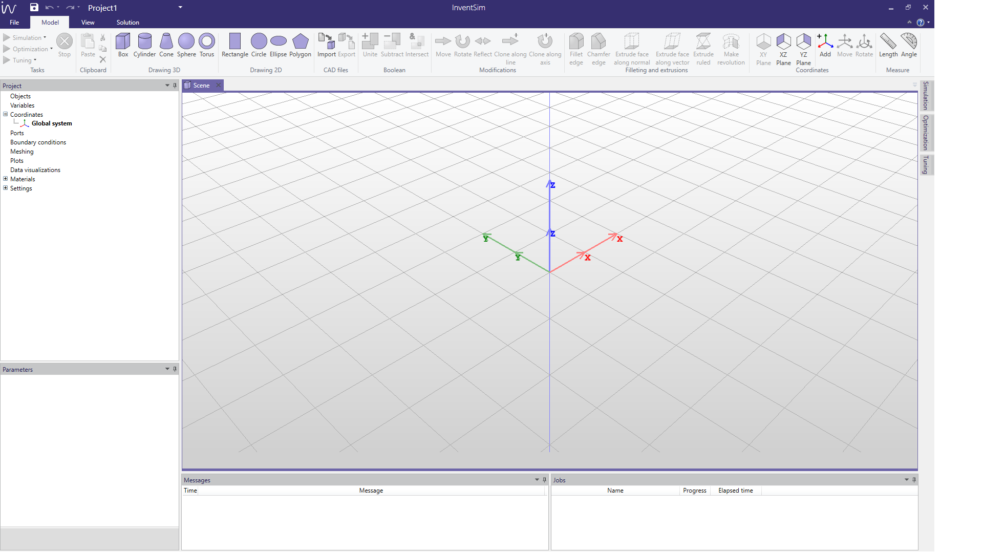
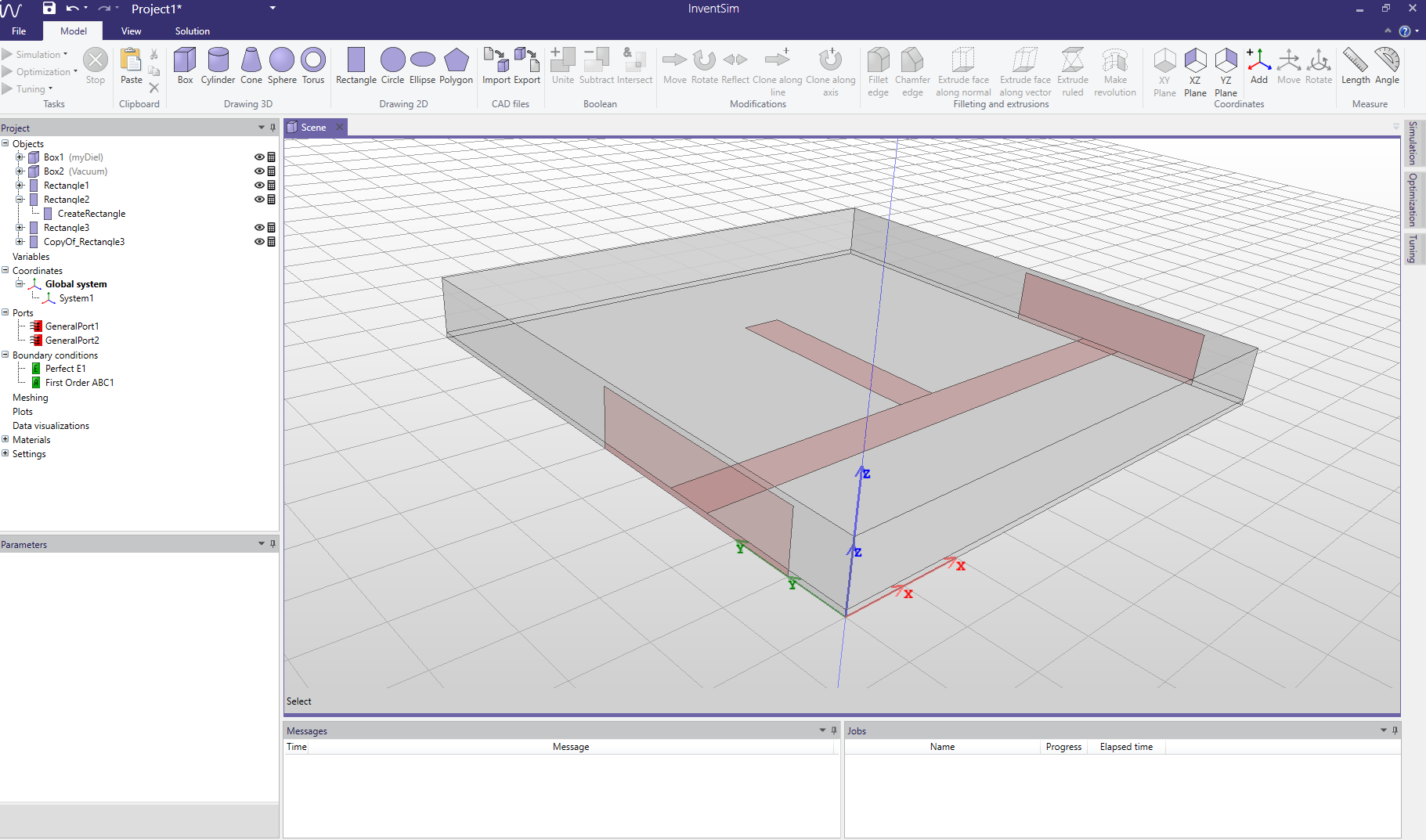
Launch InventSim and add a new, empty project. You should see a window shown in Fig 2.1:
-
• The toolbar with icons that allow you to create and manipulate objects - located on the top of the window.
-
• The tree of objects, coordinate systems, boundary conditions, field and mesh visualizations etc. located on the left.
-
• Tabs with simulation and optimization settings hidden on the right (auto-hide mode is enabled by default).
In order to define the structure we need to draw two boxes - one for the dielectric substrate and the second to model the air (vacuum) above the substrate. To start, click the box icon (
![]() ). Draw one box starting from point (0,0,0) with dimensions XDim=50, YDim=50, ZDim=0.508 - please note that the default length unit is a millimeter (mm). Draw the second box, starting from point (0,0,0.508) with
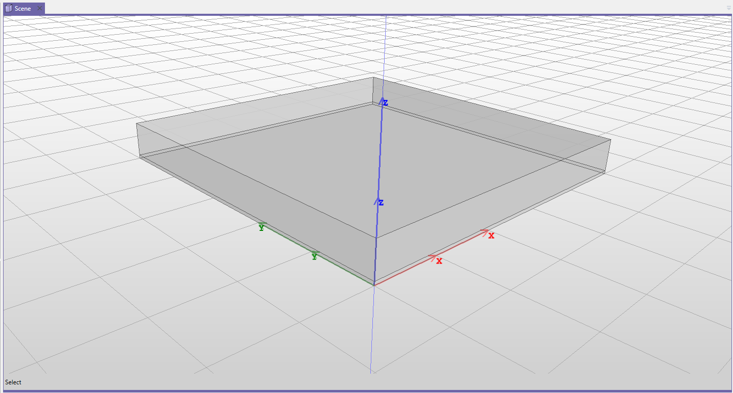
dimensions XDim=50, YDim=50, ZDim=5. The result should be as it is in Fig 2.2. Please note that the default boundary condition enforced on
the outer surfaces of our model is always that of a perfect conductor (PEC). In result, at this point both vacuum boxes are surrounded by perfectly-conducting metallic walls. The lower surface of box representing the
dielectric layer is therefore a PEC surface and constitutes a groundplane of a microstrip line.
). Draw one box starting from point (0,0,0) with dimensions XDim=50, YDim=50, ZDim=0.508 - please note that the default length unit is a millimeter (mm). Draw the second box, starting from point (0,0,0.508) with
dimensions XDim=50, YDim=50, ZDim=5. The result should be as it is in Fig 2.2. Please note that the default boundary condition enforced on
the outer surfaces of our model is always that of a perfect conductor (PEC). In result, at this point both vacuum boxes are surrounded by perfectly-conducting metallic walls. The lower surface of box representing the
dielectric layer is therefore a PEC surface and constitutes a groundplane of a microstrip line.
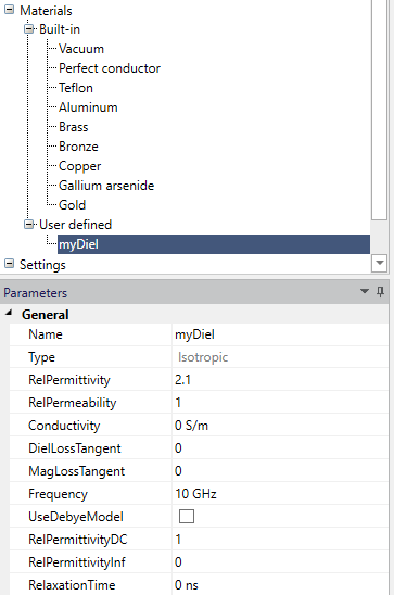
At this point, we should have two objects on the objects list (located on the left): both made of vacuum. Let us add a new dielectric material with dielectric relative permittivity equal to \(\epsilon _r=2.1\). Click the "Materials" from the project tree, click the right mouse button and select "Add->Isotropic". You can find a new position "Material1" on the list of materials. This position can be edited. Rename the position to "myDiel" and enter the relative permittivity to "2.1" as shown in Fig. 2.3. At this point, you can also change the appearance of the objects made from this material (for example, color and transparency).
Once you have added the material, you can assign it to the box representing the dielectric layer. Select the box from the objects list, click the right mouse button, select "Set material..." from the context menu and select "myDiel" from the list of available materials.
At this point you have defined a basic 3D object. The next step is to define the microstrip transmission line that will be represented as a 2D object - the rectangle located on the top of dielectric layer.
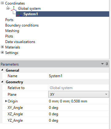
In InventSim, 2D objects are always placed on the XY, XZ or YZ planes of the current coordinate system. If you want to put a metallic strip on the upper layer of the dielectric, you need to introduce a new coordinate system that will
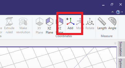
lay on the upper surface of the dielectric. Click the "Add coordinate system" icon from the upper toolbar (
![]() , Fig.2.4) and put it in location X=0, Y=0, Z=0.508 (Fig.2.5).
, Fig.2.4) and put it in location X=0, Y=0, Z=0.508 (Fig.2.5).
This new coordinate system becomes active and you are ready to draw 2D objects on top of the dielectric (plane XY in newly added coordinate system).
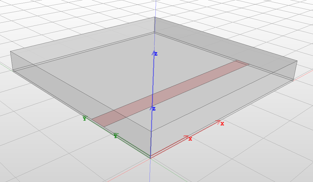
Draw a rectangle starting from point X=0, Y=13 and size it XDim=50, YDim=4 using the draw rectangle icon (
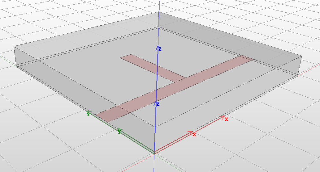
![]() ). The result is shown in Fig. 2.6. Add a section of transmission line connected in parallel to the first one (right in the middle). Draw a second
rectangle starting from point X=23, Y=17 and size it XDim=4, YDim=20. When entering the "YDim" you can also define it as a variable by entering "L=20". In that case, the variable named "L" would be added to a variables list and
initialized with value 20.
). The result is shown in Fig. 2.6. Add a section of transmission line connected in parallel to the first one (right in the middle). Draw a second
rectangle starting from point X=23, Y=17 and size it XDim=4, YDim=20. When entering the "YDim" you can also define it as a variable by entering "L=20". In that case, the variable named "L" would be added to a variables list and
initialized with value 20.
The final model of the structure is shown in Fig. 2.7.
When looking at the list of objects, it is visible that both 2D objects (rectangles) do not have any materials assigned to them. In InventSim, 2D objects do not have definable material properties like the 3D objects. Instead, you can only define boundary conditions enforced on their surface. In this case, in order to make them metallic strips, you need to select each of them, click the right mouse button and select "Set boundary condition-> Perfect E". This enforces the surface to be a perfect electric conductor. You can notice that after doing this, new elements are shown on the project tree list in the "Boundary conditions" category.
The next step is to define an excitation for our structure - in this case, it will be two wave ports on both ends of the microstrip transmission line. Draw two rectangles representing ports on the YZ plane - it is possible to select this plane using the "YZ Plane" icon from the upper toolbar. Afterwards, switch back to the global coordinate system by selecting it from the list of coordinate systems on the project tree and clicking "Activate". Now, you can draw a rectangle starting with point Y=5, Z=0 and size it YDim=20, ZDim=5. This object ("Rectangle3") will be the first port.
You can select this object from the objects tree and copy and paste it using the Ctrl+C, Ctrl+V keys. A new object named "Copy of Rectangle 3" appears, which can be moved to the opposite surface of the domain by using the "Move" operation with offset X=50, Y=0 and Z=0. Finally, select "Rectangle3", click it with the right mouse button, select "Set Port -> General Waveguide". Do the same for the other port.
You can also make the structure open from the top: select the upper surface of the object representing the air/vacuum and therefore enforcing absorbing boundary condition on it (click the right mouse button on the object, select "Pick Faces", then pick the face of the object, use the right mouse button on the object again and select "Set boundary condition -> First order absorbing").
After going through all the steps described above you should see the same structure as the one in Fig. 2.8.
2.2 Simulation setup
Once the structure geometry, materials and boundary conditions are defined, let us can move on to the simulation setup. On the right of the main InventSim window, locate the "Simulation" tab. The tab allows you to define the settings for meshing and a frequency plan.
When it comes to the mesh, you can simply restrict the maximum mesh size to not be greater then the provided value - in this case, define it as 2mm, as shown in Fig. 2.9. More advanced meshing options are described in chapter 7 1
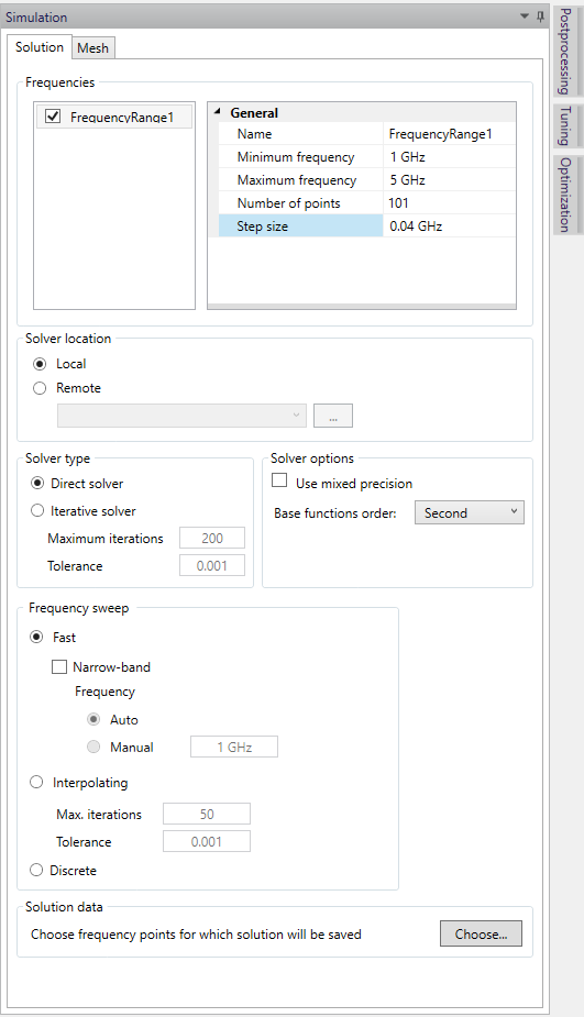
The next step is to define the frequency plan. Add one by clicking the right mouse button on the "Frequencies" box (it should be empty at this point) and select "Add". Then, assign a frequency plan: the starting frequency (1GHz), stopping frequency (5GHz) and the number of frequency points (101), as shown in Fig. 2.10.
In the lower part of the window, you can find a set of options for a fast frequency sweep. Enable this in this project and select the "Wideband" option. More on this setting can be found in chapter 8.
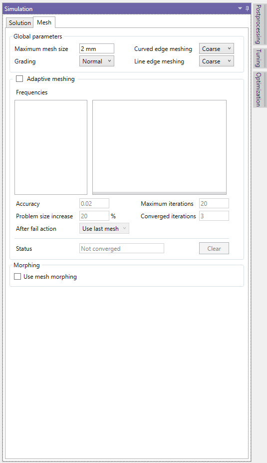
1 Please note that proper meshing is crucial for the quality of your solution and the accuracy of simulation results. In this Userguide, we perform a coarse simulation of our structure.
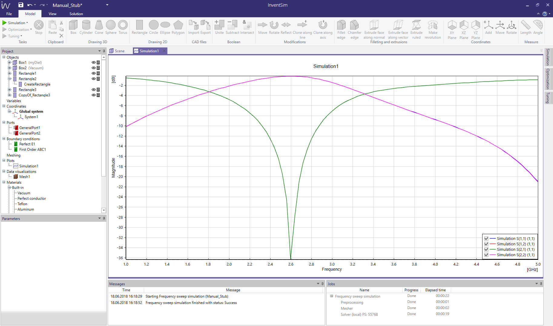
2.3 Simulation and postprocessing
The model is now ready for simulation. It is recommended to save the project on your hard drive before starting the simulation.
Once that is done, click the simulation icon on the upper left toolbar (
![]() ). The simulation will then start and the progress will be displayed on the "Messages" and "Jobs" windows at the bottom of the main InventSim window. The simulation starts with the processing of geometry, followed by the
mesh generation and the problem solution (which is usually the most computationally intensive part).
). The simulation will then start and the progress will be displayed on the "Messages" and "Jobs" windows at the bottom of the main InventSim window. The simulation starts with the processing of geometry, followed by the
mesh generation and the problem solution (which is usually the most computationally intensive part).
Once the mesh is ready, it can be displayed with the right mouse click on the 3D view window and selecting "Show mesh".
After simulating, you may add a plot of circuit response (usually, scattering parameters). Click the "Solution" tab on the upper toolbar and select "Add rectangular" to define a new plot and select data series displayed (see section 9.1) for details). You can zoom in on the plot, add markers or modify the dataseries by using the context menu with the right mouse click on the plot.
3 Geometry modeler
InventSim has the capability to construct computer models of two-dimensional and three-dimensional geometrical structures. The main part of the application is the modeler: a 3D editor that allows you to create and modify geometrical models of 3D and 2D structures.
The modeling is based on the Constructive Solid Geometry (CSG) technique. Complex geometries can be created from simple objects, known as primitives, and then modified and/or subjected to Boolean operations. For example, creating a box with a cylindrical hole in the center is achieved by creating a box first, then creating a cylinder and subtracting it from the box, as seen in the picture 3.1
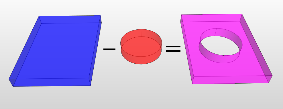
All operations on structures are parameterized: after the operations have been performed, their parameters can still be changed. For example, after creating a box, its position and dimensions can be changed without having to remove and create the box again. The operations performed on a structure form a list. It is executed from top to bottom in order to create the final structure. List of the operations can be seen as a blueprint for the structure. For example, this is the operation list of the structure seen above:
-
• Create a box.
-
• Create a cylinder in the center of the box.
-
• Subtract the cylinder from the box.
When the list is executed in that particular order, the result is a box with a hole inside it. As mentioned above, each operation is parameterized, so that position and dimensions of the box (as well as those of the cylinder) can later be changed without requiring you to recreate the entire structure. Each time you change the operation parameter, the structures rebuild themselves according to the new specification.
The modeler requires a coordinate system because it works in 3D space. It exclusively uses Cartesian right-handed coordinate systems. The default system is the global coordinate system, which cannot be deleted or modified. Other systems, which are related to the global system (or another, previously defined system), can be added. One of the coordinate systems is always active, which means that newly added operations will use that system as a reference. Each operation can have a different coordinate system assigned. Coordinate systems are parameterized in the same way as operations: changing one of the parameters causes the structure to be rebuild.
3.1 Controlling 3D view
You can move (pan), rotate and zoom the camera using the mouse, while pressing the necessary key. Normally, the middle mouse button (MMB) and mouse scroll are used to manipulate the camera, but if these are not available, you can use the right mouse button (RMB) as well. The table 1 explains how to manipulate the camera in both cases.
| Action |
With scroll/middle mouse button |
Without scroll/middle mouse button |
| Move |
Hold Ctrl and MMB while moving the mouse |
Hold Ctrl and RMB while moving the mouse |
| Rotate |
Hold MMB while moving the mouse |
Hold Ctrl+Shift and RMB while moving the mouse |
| Zoom |
Use the mouse scroll |
Hold Shift while moving the mouse |
By default, the camera rotates around the center point, which is the center for all objects, and with the Z-axis as its rotation axis. This allows you to rotate the camera around the entire scene. Alternative camera rotation mode can be enabled by moving the mouse cursor close to the left (or right) edge of the 3D View (the mouse cursor should change to "two arrows" cursor) and then rotating the view in the same way as described above. In this mode, the camera can be rotated around its own axis.
Furthermore, camera can be automatically positioned so that all structures are seen by using "Zoom to all commands" from the context menu. Similarly, the camera can be zoomed to a particular object(s) by first selecting the desired object and then clicking "Zoom to objects" from the context menu.
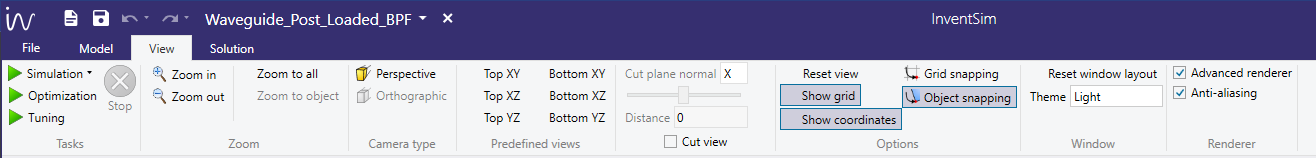
Perspective and Orthographic camera projections can be changed by selecting the appropriate button from the toolbar, as seen in Fig. 3.2.
3.1.1 Cut view
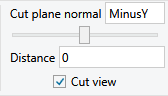
Cut view allows to render only part of the scene to better visualize some aspects of the project, for example to view internal parts of opaque objects. In order to view entire structure cut view can be enabled from the View ribbon menu by clicking on "Cut view" checkbox as shown in Fig.3.3. When enabled only part of the scene is rendered i.e. a part defined by the cut of 3D scene by a specified plane. The plane is defined by the plane normal and a distance which can be set in "Cut view" section of "View" ribbon (Fig.3.3).
3.2 Coordinate systems
The modeler uses coordinate systems to specify positions, define planes and directions in three-dimensional space. It exclusively uses Cartesian right-handed coordinate systems. The default system, named the global system cannot be modified or deleted and it is used internally by the geometry kernel. Other systems which are related to the global system (or another, previously defined system) can be added.
3.2.1 Planes
Some tools and operations require definition of the plane as a parameter value. Planes are associated with the active coordinate system which implicitly defines three planes:
-
• XY plane - the plane spanned by X and Y axes,
-
• XZ plane - the plane spanned by X and Z axes,
-
• YZ plane - the plane spanned by Y and Z axes.
Tools will use the active plane as the specified plane. Each of the planes can be chosen as the active plane by using the corresponding button from the toolbar, Fig. 3.4.

3.2.2 Directions
Some tools and operations require definition of the direction, for example rotation of objects requires definition of the axis of rotation. The direction used by the tool is the axis perpendicular to the active plane:
-
• for XY plane - Z-axis,
-
• for XZ plane - Y-axis,
-
• for YZ plane - X-axis.
3.2.3 Operations on coordinate systems
Adding
To add a coordinate system, select "Add command" from the toolbar. Specify the origin of the coordinate system by selecting the position with the mouse and clicking LMB or typing it after pressing Tab. The new coordinate system
will be relative to the previously active coordinate system. Once the system is added, its properties (like origin or rotation angles) can be modified in the parameters tab.
Moving
To move a coordinate system, i.e. change its origin, select it first and then select "Move" from the toolbar. Next, specify the new origin by selecting the position with the mouse and clicking LMB or typing it after pressing Tab.
Alternatively, enter the new origin in the parameters tab.
Rotating
To rotate a coordinate system, select the system in the project tree. Then, select the axis of rotation by selecting the correct active plane. Select "Rotate" from the toolbar. Now you can specify the angle by moving the mouse and
clicking LMB or typing it after pressing Tab. Alternatively, enter the new angle in the parameters tab.
Deleting To delete a coordinate system, select it in the project tree and then select "Delete" from the context menu. Coordinate systems used by an object cannot be deleted. In such a case, an error message will be shown.
3.3 Objects
The main part of the application is the modeler, a 3D editor allowing you to create and modify geometrical models of 3D and 2D structures. The modeler has the capability to model one, two and three-dimensional geometrical structures in 3D space.
The modeling is based on the Constructive Solid Geometry (CSG) technique. Complex geometries can be created from simple objects, known as primitives, and then modified and/or subjected to Boolean operations. For example, creating a box with a cylindrical hole in the center is achieved by creating a box first, then creating a cylinder and subtracting it from the box, as seen in the picture below.
All operations on structures are parameterized: after the operations have been performed, their parameters can still be changed. For example, after creating a box, its position and dimensions can be changed without having to remove and create the box again. The operations performed on a structure form a list, which is executed from top to bottom in order to create the final structure. List of operations can be seen as a blueprint for the structures. For example, this is the operations list of the structure seen above: Create a box. Create a cylinder in the center of the box. Subtract the cylinder from the box. When it is executed in that particular order, it results with a box with a hole in it. As mentioned above, each operation is parameterized, so that the position and dimensions of the box (as well as those of the cylinder) can later be changed without requiring you to recreate the entire structure. Each time you change the operation parameter, the structures rebuild themselves according to the new specification.
The purpose of the modeler is to model geometrical structures. Structures are divided into logical entities called SimObjects: one is made of structures of the same category (only solids, only faces or only one-dimensional objects) that share some of properties. For example all solids in a SimObject are assumed to be made of the same material.
3.3.1 Primitives
The building blocks of every modeled object are primitives, grouped in three categories. The first one is the three-dimensional closed solids, for which the available primitives are:
-
• Box
-
• Cylinder
-
• Cone
-
• Sphere
-
• Torus
The other category is the two-dimensional flat faces, and the list of primitives is as follows:
-
• Rectangle
-
• Circle
-
• Ellipse
-
• Polygon
Finally, the last group are 1D objects:
-
• Line
-
• Polyline
-
• B-spline
-
• Arc of circle
Each primitive can be constructed by selecting an appropriate tool from the toolbar (Fig.3.5. For example, creating a box requires the "Box" tool from the "Drawing 3D" toolbar section. The tools are interactive and the parameters of a particular object are set using either the mouse or pressing Tab and typing the exact values.
New objects are added with the "Create" operation located at the top of operations list. These operations are responsible for constructing objects and defining their geometrical parameters, i.e. its origin (common parameter P0) or its dimensions.
When selecting a drawing tool, the active coordinate system as well as the active plane of that system are used as appropriate parameter values of the "Create" operation.
To properly model 2D objects, InventSim requires them to be drawn on the surfaces or walls associated to 3D objects!
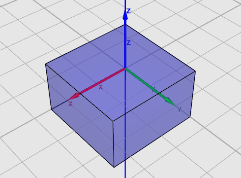
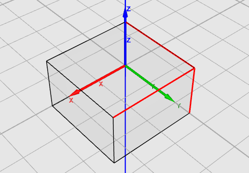
3.3.2 Box
A box is defined as a cuboid with its faces parallel to the coordinate system axes. To add a box, select the "Box" tool, specify its origin and then specify its X, Y and Z dimensions (Fig.3.6).
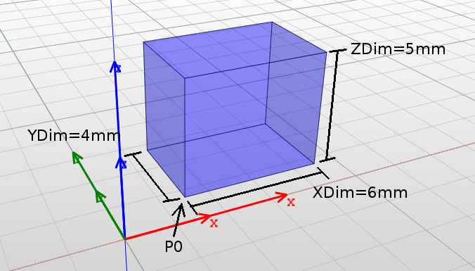
Boxes are constructed by CreateBox operation and the parameters are:
-
• Coordinate System: Assigned coordinate system.
-
• Plane: Irrelevant for the box.
-
• P0: Origin of the box: the position of one of its corners.
-
• XDim: Width of the box in X-axis.
-
• YDim: Width of the box in Y-axis.
-
• ZDim: Width of the box in Z-axis.
Remarks:
-
• Faces are parallel to the coordinate system axes and cannot be skewed.
-
• Width values can be negative. In such a case the box will be created as if the corresponding axis had the opposite direction.
-
• Faces name correspond to coordinate system planes: BottomXY and TopXY for faces parallel to XY plane, BottomXZ and TopXZ parallel to XZ plane, BottomYZ and TopYZ parallel to YZ plane.
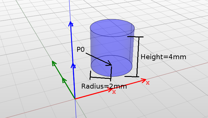
3.3.3 Cylinder
A cylinder is defined as a solid that has two parallel, circular bases connected by a curved surface. The orientation of the cylinder, i.e. its axis, is set as the direction perpendicular to the active plane of the active coordinate system. To add a cylinder, select the "Cylinder" tool, specify its origin and then specify its radius and height (Fig.3.7).
Cylinders are constructed by CreateCylinder operation and the parameters are:
-
• Coordinate System: Assigned coordinate system.
-
• Plane: Defines the axis of the cylinder, which is a vector normal to the active system plane.
-
• P0: Origin of the cylinder: the center of its bottom base.
-
• Radius: Radius of the cylinder.
-
• Height: Height of the cylinder: its length along the axis.
Remarks:
-
• The axis of the cylinder is perpendicular to the plane of the coordinate system and cannot be changed.
-
• Height can be negative. In such a case the cylinder will be created as if the axis had the opposite direction.
-
• Radius must not be negative.
-
• Face name are: BottomBase and TopBase for cylinder bases and Side for cylindrical face.
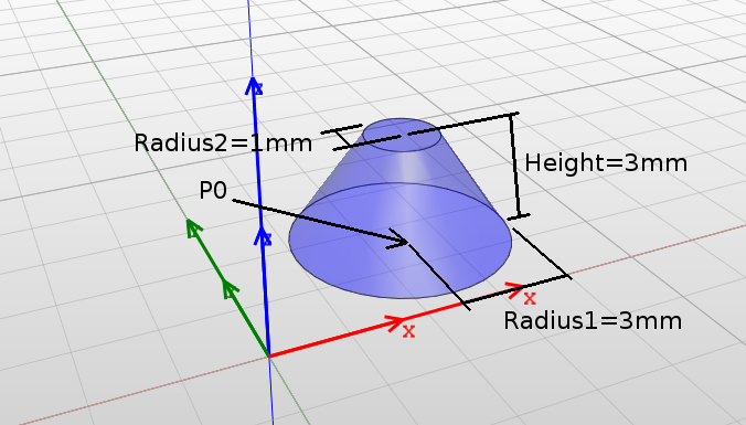
3.3.4 Cone
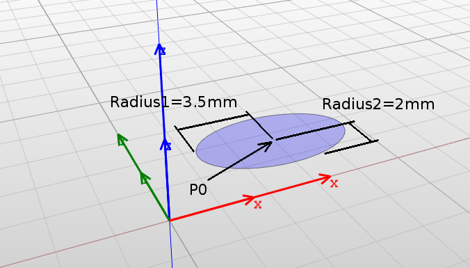
A cone is defined as a solid that tapers smoothly from a flat, circular base to a point or another base (truncated cone). The axis of the cone is perpendicular to the base and is set as the direction perpendicular to the active plane of the active coordinate system. To add a cone, select the "Cylinder" tool, specify its origin and then specify the radii of the bottom and the base (Fig.3.8).
Cones are constructed by CreateCone operation and the parameters are:
-
• Coordinate System: Assigned coordinate system.
-
• Plane: Defines the axis of the cone, which is a vector normal to the system active plane.
-
• P0: Origin of the cone: the center of its bottom base.
-
• Radius1: Radius of the bottom base.
-
• Radius2: Radius of the top base.
-
• Height: Height of the cone: its length along the axis.
Remarks:
-
• The axis of the cone is perpendicular to the plane of the coordinate system and cannot be changed.
-
• Height can be negative. In such a case the cone will be created as if the axis had the opposite direction.
-
• Neither Radius1 nor Radius2 can be negative.
-
• Face name are: BottomBase and TopBase for cone bases and Side for conical face.
3.3.5 Sphere
A sphere is defined as a solid with one face, which is a set of all points that are located at a certain distance (radius) from a point (origin). To add a sphere, select the "Sphere" tool and specify its origin and radius (Fig.3.9).
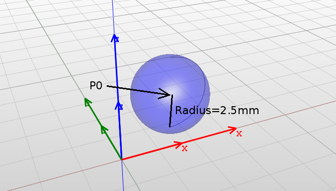
The spheres are constructed by CreateSphere operation and the parameters are:
-
• Coordinate System: Assigned coordinate system.
-
• Plane: Irrelevant for the sphere.
-
• P0: Origin of the sphere: its center.
-
• Radius: Radius of the sphere.
Remarks:
-
• Radius must not be negative.
-
• Face name is SphereFace.
3.3.6 Torus
A torus is defined as a solid with one face, which is created as a surface of revolution by revolving a circle around an axis. The axis is perpendicular to the active plane of the active coordinate system and the center of revolution is the torus origin point. To add a torus, select the "Torus" tool and specify its origin and both radii.
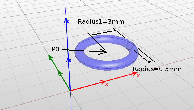
Toruses are constructed by CreateTorus operation and the parameters are:
-
• Coordinate System: Assigned coordinate system.
-
• Plane: Defines axis of the torus which is a vector normal to the system active plane.
-
• P0: Origin of the torus: its center.
-
• Radius1: Radius of the torus: distance from the origin to the center of revolving circle.
-
• Radius2: Radius of the toroidal face.
Remarks:
-
• Neither Radius1 nor Radius2 can be negative.
-
• Face name is Torus.
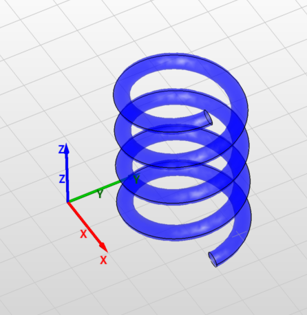
3.3.7 Helix
A helix is defined as a solid with one face, which is created as a surface of revolution by revolving a circle around an axis. The axis is perpendicular to the active plane of the active coordinate system and the center of revolution is the torus origin point. To add a torus, select the "Torus" tool and specify its origin and both radii.
Helices are constructed by CreateHelix operation and the parameters are:
-
• Coordinate System: Assigned coordinate system.
-
• Plane: Defines axis of the helix which is a vector normal to the system active plane.
-
• P0: Origin of the helix, the point on bottom end of the helix axis.
-
• Radius1: Radius of the bottom end.
-
• Radius2: Radius of the top end.
-
• Turns: Number of helix turns.
-
• Angle: Helix angle.
-
• Profile radius: Radius of the helix profile.
-
• Twist: Helix twist direction.
Remarks:
-
• Neither Radius1 nor Radius2 can be negative.
-
• Faces names are: HelixFace0 and HelixFace2 for bottom and top faces respectively, HelixFace1 for the side face.
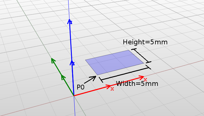
3.3.8 Rectangle
A rectangle is defined as a two-dimensional face with two pairs of edges and four right angles. The face lies on an active plane of the active coordinate system (XY, XZ or YZ). To add a rectangle, select the "Rectangle" tool, specify its origin and then specify width and height (Fig.3.12).
Rectangles are constructed by CreateRectangle operation and the parameters are:
-
• Coordinate System: Assigned coordinate system.
-
• Plane: Defines the plane on which the face lies.
-
• P0: Origin of the rectangle: position of one of its corners.
-
• Width: Length of the rectangle in the first dimension.
-
• Height: Length of the rectangle in the second dimension.
Remarks:
-
• Width and Height are defined as lengths in the first and the second dimensions of the plane. For example, if the XZ plane is set, Width is the length in X dimension and Height is the length in Z dimension.
-
• Width and Height can be negative. In such a case the rectangle will be created as if the axis had the opposite direction.
-
• 2D objects are always created on XY, XZ or YZ planes and can later be moved to other locations using the "Move" operation.
-
• Face name is Rectangle.
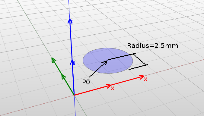
3.3.9 Circle
A circle is defined as a two-dimensional face bounded by one, circular edge. The face lies on a plane parallel to the active plane of the active coordinate system. To add a circle, select the "Circle" tool and specify its origin and radius (Fig.3.13).
Circles are constructed by CreateCircle operation and the parameters are:
-
• Coordinate System: Assigned coordinate system.
-
• Plane: Defines the plane on which the face lies.
-
• P0: Origin of the circle: its center.
-
• Width: Length of the circle in the first dimension.
-
• Height: Length of the circle in the second dimension.
Remarks:
-
• Radius must not be negative.
-
• Face name is Circle.
3.3.10 Ellipse
An ellipse is defined as a two-dimensional face bounded by an ellipse edge. The face lies on a plane parallel to the active plane of the active coordinate system. To add an ellipse, select the "Ellipse" tool and specify its origin and both radii (Fig.3.14).
Ellipses are constructed by CreateEllipse operation and the parameters are:
-
• Coordinate System: Assigned coordinate system.
-
• Plane: Defines the plane on which the face lies.
-
• P0: Origin of the ellipse: its center.
-
• Width: Length of the ellipse in the first dimension.
-
• Height: Length of the ellipse in the second dimension.
Remarks:
-
• Radius1 and Radius2 are defined as length in the first and the second dimensions of the plane. For example, if the XZ plane is set, Radius1 is the length in X dimension and Radius2 is the length in Z dimension.
-
• Radius1 and Radius2 must not be negative.
-
• Face name is Ellipse.
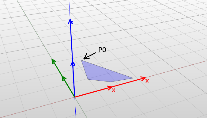
3.3.11 Polygon
A polygon is defined as a two-dimensional face bounded by a set of straight edges. Only simple polygons are allowed i.e. polygons that do not intersect themselves and have no hole. The face lies on a plane parallel to the active plane of the active coordinate system.
To add a polygon, select the "Polygon" tool and specify its origin as well as the remaining polygon vertexes: press Shift+Enter to finish adding vertexes (Fig.3.15).
Additionally regular polygons can be created by specifying the origin, one of the vertices and the number of sides.
Polygons are constructed by CreatePolygon operation and the parameters are:
-
• Coordinate System: Assigned coordinate system.
-
• Plane: Defines the plane on which the face lies.
-
• P0: Origin of the polygon: position of one of its corners.
-
• Number of points: Number of vertexes (read-only).
-
• Points: List of the positions of vertexes.
Remarks:
-
• List of vertex positions cannot be changed, only the position values can be.
-
• Face name is either RegularPolygon or Polygon.
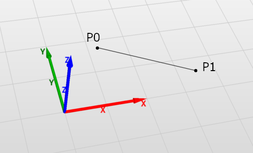
3.3.12 Line
A line is a straight line segment connecting two points. The line lies on a plane parallel to the active plane of the active coordinate system.
To add a line, select the "Line" tool and specify its two points (Fig.3.16).
Lines are constructed by CreateLine operation and the parameters are:
-
• Coordinate System: Assigned coordinate system.
-
• Plane: Defines the plane on which the line lies.
-
• P0: start point.
-
• P1: end point.
Remarks:
-
• Edge name is Line.
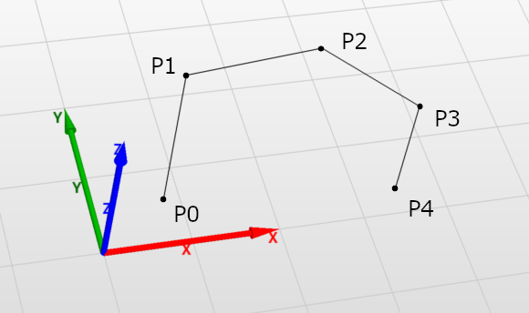
3.3.13 Polyline
Polylines are sets of connected straight line segments connecting defined points. Polylines lie on a plane parallel to the active plane of the active coordinate system.
To add a polyline, select the "Polyline" tool and specify its points (Fig.3.17).
Polylines are constructed by CreatePolyline operation and the parameters are:
-
• Coordinate System: Assigned coordinate system.
-
• Plane: Defines the plane on which the line lies.
-
• Number of points: cannot be changed after polyline is created.
-
• Points: collection of points which are connected by lines.
Remarks:
-
• Edge names are PolyLine_PartN where N is the index of the edge (starting with 0).
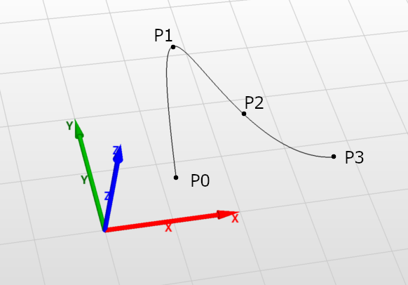
3.3.14 B-spline
In InventSim B-spline is a collection of piecewise polynomial curves passing through an array of points. It lies on a plane parallel to the active plane of the active coordinate system.
To add a B-spline, select the "B-spline" tool and specify its points (Fig.3.18).
B-splines are constructed by CreateBSpline operation and the parameters are:
-
• Coordinate System: Assigned coordinate system.
-
• Plane: Defines the plane on which the edge lies.
-
• Number of points: cannot be changed after B-spline is created.
-
• Points: collection of points which are connected by splines.
-
• Is periodic: if set BSpline curve will be periodic and closed. In this case, the junction point is the first point of the Points.
Remarks:
-
• There must be at least two points.
-
• Edge name is "BSpline".
3.3.15 Arc of circle
InventSim allows to create sections of circle in several ways depending on what parameters are more convenient for the user. The options are:
-
• Center, radius and angles
-
• Center, start and end
-
• Three points
-
• Start, end and radius
-
• Start, end and angle - makes an arc of circle from two points i.e. starting and end point and an angle formed by lines connecting the circle center and the two points.
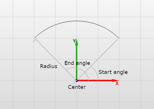
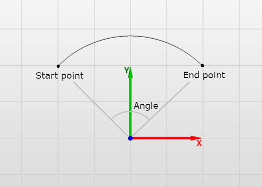
Makes an arc of circle from a circle (defined by its center and radius) and two angles. The arc spans between two points: start point and end point. Both points are calculated based on center of the circle and angles formed by the primary axis of the coordinate system and the lines connecting the starting point and the end point with the center.
To add a arc of circle, select the "Arc of circle" tool, then "Center, radius and angles" tool mode.
The arc is constructed by CreateArcOfCircle operation and the parameters are:
-
• Coordinate System: Assigned coordinate system.
-
• Plane: Defines the plane on which the curve lies.
-
• Definition: cannot be changed after arc of circle is created.
-
• Center point: center of the circle.
-
• Radius: radius of the circle.
-
• Start angle: angle between first plane axis and line connecting circle center with start point of the arc.
-
• End angle: angle between first plane axis and line connecting circle center with end point of the arc.
Remarks:
-
• Radius must be positive.
-
• Curve name is "ArcOfCircle".
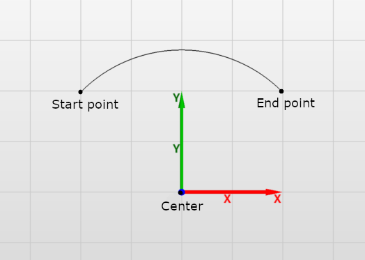
Makes an arc of circle from a circle (defined by its radius) and two points being start and end point.
To add a arc of circle, select the "Arc of circle" tool, then "Center, start and end" tool mode.
The arc is constructed by CreateArcOfCircle operation and the parameters are:
-
• Coordinate System: Assigned coordinate system.
-
• Plane: Defines the plane on which the curve lies.
-
• Definition: cannot be changed after arc of circle is created.
-
• Center point: center of the circle.
-
• Start point: start point of the arc.
-
• End point: end point of the arc.
Remarks:
-
• Curve name is "ArcOfCircle".
Make an arc of circle which spans between two points and having circle radius calculated based on a third point located on the arc between the first two points.
To add a arc of circle, select the "Arc of circle" tool, then "Center, radius and angles" tool mode.

The arc is constructed by CreateArcOfCircle operation and the parameters are:
-
• Coordinate System: Assigned coordinate system.
-
• Plane: Defines the plane on which the curve lies.
-
• Definition: cannot be changed after arc of circle is created.
-
• Start point: start point of the arc.
-
• End point: end point of the arc.
-
• Arc point: point located on the arc between start and end points.
Remarks:
-
• Curve name is "ArcOfCircle".
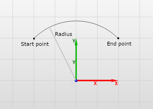
Makes an arc of circle from two points i.e. start and end point and the circle radius.
To add a arc of circle, select the "Arc of circle" tool, then Start, end and radius" tool mode.
The arc is constructed by CreateArcOfCircle operation and the parameters are:
-
• Coordinate System: Assigned coordinate system.
-
• Plane: Defines the plane on which the curve lies.
-
• Definition: cannot be changed after arc of circle is created.
-
• Start point: start point of the arc.
-
• End point: end point of the arc.
-
• Radius: radius of the circle.
-
• Positive angle:
Remarks:
-
• Curve name is "ArcOfCircle".
Makes an arc of circle from two points i.e. start and end point and an angle between lines connecting start and end points with the circle center.
To add a arc of circle, select the "Arc of circle" tool, then "Start, end and angle" tool mode.
The arc is constructed by CreateArcOfCircle operation and the parameters are:
-
• Coordinate System: Assigned coordinate system.
-
• Plane: Defines the plane on which the curve lies.
-
• Definition: cannot be changed after arc of circle is created.
-
• Start point: start point of the arc.
-
• End point: end point of the arc.
-
• Angle: angle between lines connecting start and end points with the circle center.
Remarks:
-
• Curve name is "ArcOfCircle".
3.3.16 Face from closed contour
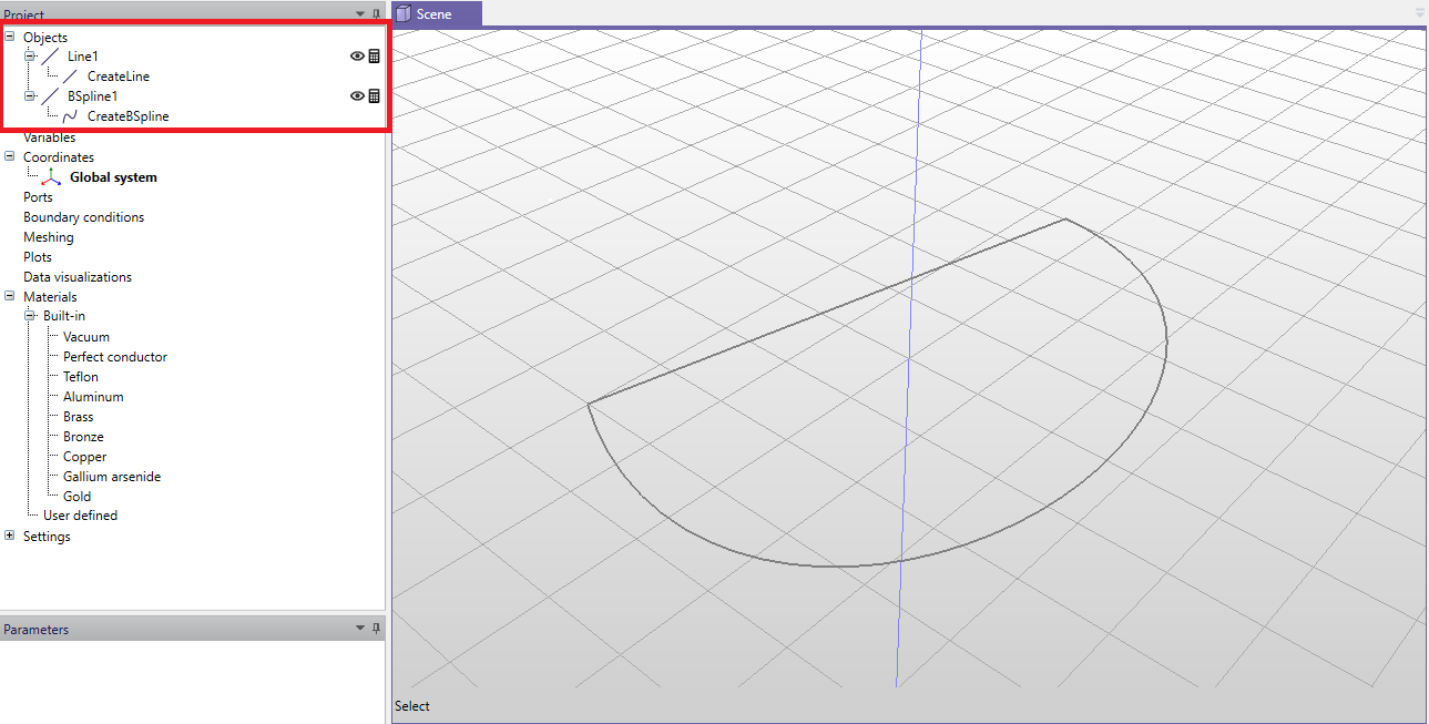
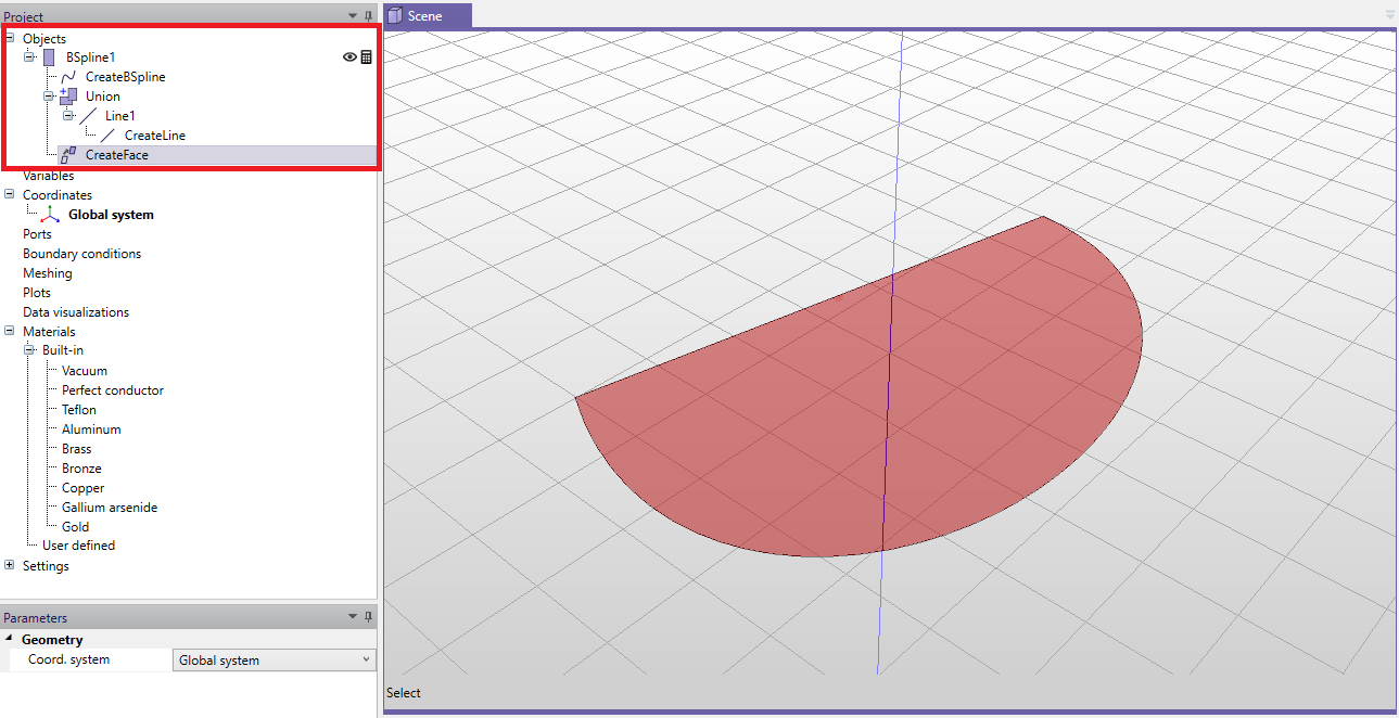
When the user draws a closed contour using 1D drawing tools, it is possible to transform it to 2D face. To use this feature, draw a contour that can consist of several 1D objects, as shown in Fig. 3.24. Then, unite the 1D objects into one closed contour, select it and click icon make face (
![]() ). The result of this operation is a 2D face, as shown in Fig. 3.25.
). The result of this operation is a 2D face, as shown in Fig. 3.25.
3.4 Boolean operations
To create geometry models that are more complex than the simple primitives, Boolean operations should be used. Boolean operations available in the modeler are an extrapolation of Boolean algebra of sets.
Notice: When using Boolean operations on the objects, all arguments of Boolean operations are deleted - only the the resulting object of the operation is stored. In order to keep the copies of those argument objects please hold "Shift" when clicking the operation icon.
3.4.1 Union
This tool creates a union of two or more objects - i.e. it merges two or more objects together. If the two objects are disjoint, the result will be an object with two separate parts. The operation can be described by the following equation:
\(\seteqnumber{0}{}{2}\)\begin{equation} A_R = A_1 + A_2 + ... + A_n \end{equation}
where \(A_R\) is the operation result and \(A_i\), (\(i=1,2,\ldots , n\)) are the operation arguments.
In order to unite two or more objects, select them, then select the "Unite" tool from the toolbar. The order in which objects are selected is not relevant.
3.4.2 Subtraction
This tool creates a difference of two or more objects - i.e. it subtracts one or more objects from a single object. The operation can be described by the following equation:
\(\seteqnumber{0}{}{3}\)\begin{equation} A_R = A_1 - A_2 - ... - A_n \end{equation}
where \(A_R\) is the operation result and \(A_i\), (\(i=1,2,\ldots , n\)) are the operation arguments.
In order to subtract two or more objects from a desired object, select it first. Then select the object(s) you wish to subtract. After that, select the "Subtract" tool from the toolbar. The order of your selection is important. The object from which you want to subtract must be selected first. Then the rest of objects can be selected.
3.4.3 Intersection
This tool creates an intersection of two or more objects - i.e. it creates an object(s) which consists of the common part of the selected objects. The operation can be described by the following equation:
\(\seteqnumber{0}{}{4}\)\begin{equation} A_R = A_1 \times A_2 \times ... \times A_n \end{equation}
where \(A_R\) is the operation result and \(A_i\), (\(i=1,2,\ldots , n\)) are the operation arguments.
In order to intersect two or more objects, select them, then select the "Unite" tool from the toolbar. The order in which the objects are selected is not relevant.
3.5 Modifications
Thanks to parametrization of objects, structures can be modified after their construction by changing the values of their parameters. Nevertheless, a set of modification tools is available for additional modifications. Using the tools requires selecting the object which will be the subject of the modification. After specifying the modification parameters values, an appropriate operation will be added to the objects operations list.
3.5.1 Move
This tool moves the object by a specified offset, defined as a three-dimensional vector. To move an object, select it first and then select the "Move" tool from the toolbar. To move the object, specify the starting point and the final point of the movement.
Moving object is performed by the "Move" operation which has the following parameters:
-
• Coordinate System: Assigned coordinate system.
-
• Offset: Offset by which the object is moved.
3.5.2 Rotate
This tool rotates the object by a specified angle around an axis. The axis is determined by the active coordinate system and the active plane upon selecting the tool. It is set as the direction perpendicular to the active plane with the center of rotation being the origin of the active coordinate system. For example, if the YZ plane is the active plane, the axis will be a vector parallel to X-axis. To rotate the object, select it first and then select the "Rotate" tool from the toolbar. Specify the angle of rotation either by moving the mouse and clicking LMB or by typing the exact value after pressing Tab.
Rotation of objects is performed by the "Rotate" operation which has the following parameters:
-
• Coordinate System: Assigned coordinate system.
-
• Plane: Determines the axis of rotation.
-
• Angle: Angle of rotation.
3.5.3 Reflect
This tool reflects an object across a specified plane. To reflect an object, select it first and then select the "Reflect" tool from the toolbar. Specify the plane of rotation by moving the mouse over 3D View and click LMB.
Reflecting object is performed by the "Reflect" operation which has the following parameters:
-
• Coordinate system: Assigned coordinate system.
-
• Plane: Plane by which the object is reflected.
3.5.4 Clone along line
This tool takes an object and creates one (or more) exact copy of it. The cloned objects are placed along a specified line, each displaced by a specified distance. Construction of the clones is done by the CreateByCloning operation which is added to the top of the clones operations list. Any changes to the original object operations parameters prior to cloning will result in reconstruction of the clones.
To clone an object along a line, select it and then select "Clone along line tool" from the toolbar. Determine the displacement of the clones by specifying the starting and the final points and then enter the wanted number of clones.
Cloning along line is performed by "CloneAlongLine" operation which has the following parameters:
-
• Coordinate System: Assigned coordinate system.
-
• Copies: Number of created clones.
-
• Offset: Offset by which each of the clones is displaced.
Remarks:
-
• Clones are completely independent - i.e. modifying or deleting one of the clones will not affect the rest of the clones, nor the original object.
-
• Deleting the original object does not affect the clones.
-
• Deleting CloneAlongLine operation from the original object operations list removes all the clones.
3.5.5 Clone around axis
This tool takes an object and creates one (or more) exact copy of it. The clones are placed around a specified point, each rotated by a specified angle. The axis is determined by the active coordinate system and the active plane upon selecting the tool. It is set as the direction perpendicular to the active plane with the center of rotation being the origin of the active coordinate system. Construction of the clones is done by CreateByCloning operation which is added to the top of the clones operations list. Any changes to original object operations parameters prior to cloning results in reconstruction of the clones.
To clone an object around axis, select it first and then select "Clone around axis" tool from the toolbar. Specify the angle of rotation either by moving the mouse and clicking LMB or by typing the exact value after pressing Tab key and then entering the number of clones.
Cloning around axis is performed by "CloneAroundAxis" operation which has the following parameters:
-
• Coordinate System: Assigned coordinate system.
-
• Copies: Number of created clones.
-
• Plane: Determines the axis of rotation.
-
• Angle: Angle by which each of the clones is rotated.
Remarks:
-
• Clones are completely independent - i.e. modifying or deleting one of the clones will not affect the rest of the clones nor the original object.
-
• Deleting the original object does not affect the clones.
-
• Deleting CloneAroundAxis operation from the original object operations list removes all the clones.
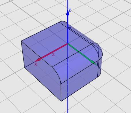
3.5.6 Fillet edge
This tool creates fillets which are the rounding of the edges of solids. To use the tool, select "Pick edges" and then select one or more edges. Use the toolbar and select "Fillet edge". You will be asked for the radius of the fillet (Fig.3.26).
Remarks:
-
• If the fillet cannot be created or fails to generate, the result will be equivalent to Radius=0.
-
• Creating fillets on some edges will result in having fillets on other edges.
3.5.7 Edge chamfering
This modification is similar to edge filleting, but the edges are cut as opposed to being rounded. (Fig.3.27).
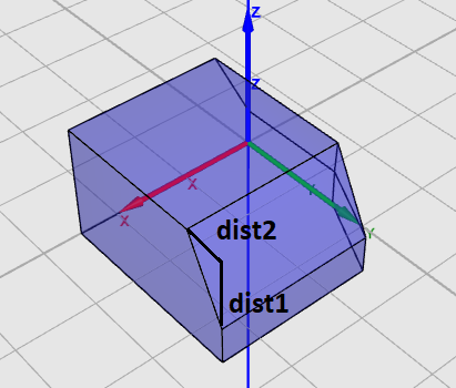
Edge chamfering is performed by "ChamferEdge" operation which has the following parameters:
-
• Coordinate System: Assigned coordinate system.
-
• Dist1: Distance from one edge to be cut.
-
• Dist2: Distance from the other edge to be cut
3.5.8 Extrude
Extruding is an operation that modifies the 2D object into a solid. Three variants of extrusion are available in InventSim:
-
• Extrude along normal: It is the simplest variant, where the 2D object is extruded along a vector normal to its surface. For example, extrusion of a rectangle would give you a box.
-
• Extrude along vector: In this case the extrusion is made along an arbitrary, used-defined vector.
-
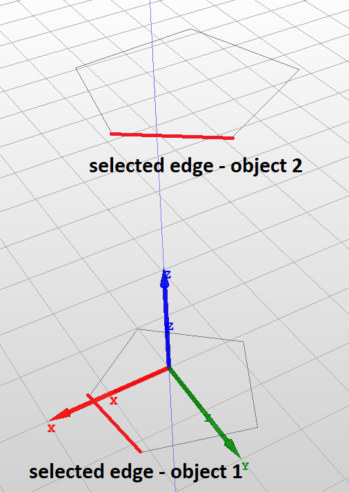
• Extrude ruled: With this operation, is is possible to construct a solid with a ruled surface. To do so, the user needs to provide two 2D objects with the same number of edges and then select one edge in each object (Fig. 3.28). The operation would connect the nodes of the objects with straight lines.
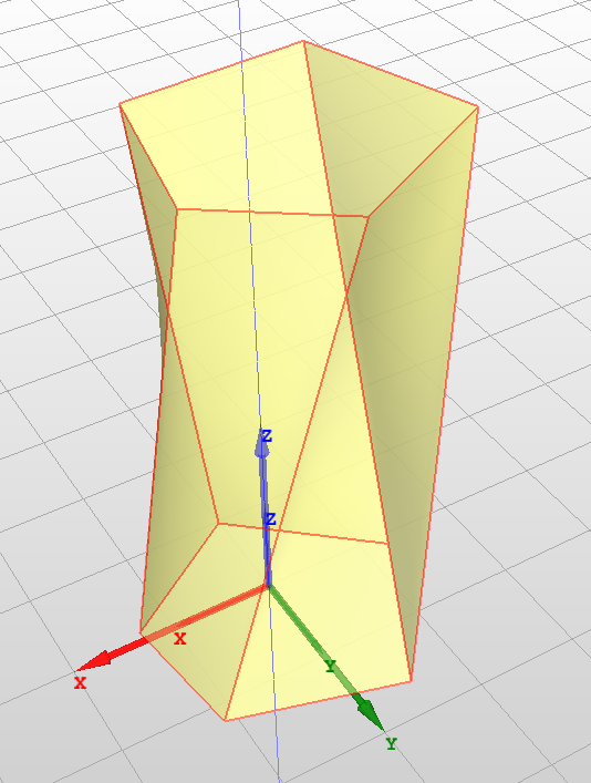
3.5.9 Revolution around axis
The revolution operation transforms a 2D object into a 3D solid by rotating the surface around an axis of rotation.
The "Revolution" operation has the following parameters:
-
• Coordinate System: Assigned coordinate system.
-
• Plane: Plane of rotation
-
• Angle: Angle of rotation
Remarks:
-
• 2D object can not lay down on the plane of rotation.
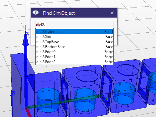
3.6 Selecting objects
To access the object properties, modify object faces or edges, you need to select proper object, its face or edge. This can be done using the mouse, but also with the special dialog box "Find SimObject" accessible with "Ctrl+T" shortcut (Fig. 3.29).
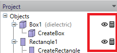
3.7 Hiding and disabling calculation of objects
By using the icons on the object list in the project tree panel (Fig.3.30, you can easily control the properties of the object, such as:
-
• Visibility: select this icon (
 ) to enable/disable object display in the 3D view window.
-
• Activity: select this icon (
 ) to exclude the object from calculations (object is still visible in the 3D view, but is not taken into account during simulations).
3.8 Variables and equations
One of the basic features of InventSim is model parametrization by using variables. This feature is essential for efficient and successful design, since it allows you to change and control the model geometry in an easily accessible way. In principle, there are algebraic expressions which, when evaluated, represent floating point values. Variables may be used as values of most of the parameters - instead of numerical values. Whenever a variable value changes, objects that use that variable are reconstructed with the new parameters values.
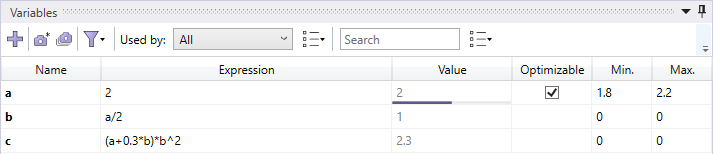
The variables are available in the variables panel, located by default below the scene view (Fig. 3.31). The panel presents all variables in a table form where each row shows parameters of a single variable. Above the table a toolbar is shown providing additional functionalities described below.
3.8.1 Adding variables
There are several ways to add a new variable:
-
• Right click on the "Variables" and select "New" from the context menu. A new variable will be added to the list of variables with the default name and the value of zero - the user can then modify the name and assign the value of the variable using the variable properties window.
-
• Click
 button in the toolbar.
-
• When creating/modifying an object and entering its dimensions you can input a string with the variable name and its value, for example entering the string "b=10.16" as the box size parameter "YDim"
-
• When creating/modifying an object and entering its dimensions you can input a string with the name of the variable. (for example "c") When no variable with that name is found, you will be asked about the value of that variable, as shown in Fig. 3.32.
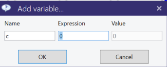
The variables can later be used in formulas (equations) that use the already defined variables. For example, if variables "a" and "b" exist within the project, we can enter an equation "c = a + b/2". Several mathematical functions can be used in the expression, like trigonometric functions \(sin(), cos()\) - a full list is shown in table 2. Predefined constants are shown in table 3.
3.8.2 Deleting variables
To delete a variable use one of the following actions:
-
• Select the variable from the list and press "Del" keyboard button.
-
• Select the varaible from the list and select "Delete" from the context menu.
Note that only unused variables can be deleted. An attempt to delete a referenced variable will result in an error.
3.8.3 Sorting and filtering
Variables list can be sorted by any of the parameters shown by clicking on a column header. By default the order in which variables are shown is the order in which they were added. Clicking one the column header sorts variables by that column in ascending order. Second click reverses sorting and the third resets sorting.
Additionally variables can be filtered in several ways to show:
-
• only optimizable variables
-
• only variables used in a particular object, coordinate system or material,
-
• only variables containing a specified text.
To show only optimizable variables click on
 button in the toolbar and check "Only optimizable" checkbox.
To display only variables used in the parameter values of a specific object, coordinate system, or material, select that object from the "Used by" drop-down list. Select "All" if you want to clear the filter. Additionally, a drop-down options menu is available where the user can specify the context in which variables are used. The "Include equations" option means that nested variables used in equations referenced in parameter values will also be shown. For example, if two variables are present, "a=1" and "b=a/2," and an object uses the variable "b," variable "a" will also be shown because it is used in the equation defining variable "b." The "Include coordinate systems" option allows including variables used in all coordinate systems referenced by the selected object.
To show only variables containing certain text, type that text in the "Search" text box. The options drop-down menu allows you to specify where the text will be searched: variable names and/or variable equations.
3.8.4 Variable snapshots
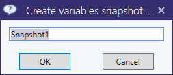
InventSim allows users to store sets of variable values for later use. These sets are called snapshots and contain all real valued variable values. To create and add a snapshot click on
 button in the toolbar. A dialog prompting for a snapshot name will appear (Fig.3.33). Click "OK" button to confirm the name and
add the snapshot. To view stored snapshots click on
button in the toolbar. A dialog prompting for a snapshot name will appear (Fig.3.33). Click "OK" button to confirm the name and
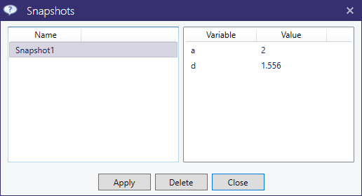
add the snapshot. To view stored snapshots click on
 button in the toolbar. Snapshots view will appear in a dialog window as shown in Fig.3.34. To delete a snapshot, select it in the left
pane and click on "Delete" button. To apply snapshot, select it in the left pane and click on "Apply" button.
button in the toolbar. Snapshots view will appear in a dialog window as shown in Fig.3.34. To delete a snapshot, select it in the left
pane and click on "Delete" button. To apply snapshot, select it in the left pane and click on "Apply" button.
3.8.5 Functions
| Symbol | Description |
| ̂ | Power |
| + | Add |
| - | Subtract |
| / | Divide |
| * | Multiply |
| cos() | Cosinus |
| sin() | Sinus |
| exp() | Exponential |
| ln() | Natural logarithm |
| tan() | Tangent |
| acos() | Arcus cosinus |
| asin() | Arcus sinus |
| atan() | Arcus tangent |
| sqrt() | Square root |
| cotan() | Cotangent |
| acotan() | Arcus cotangent |
| round(a, PRECISION) | Round number up to provided precision |
| ceil() | Smallest following integer |
| floor() | Largest previous integer |
| abs() | Module |
| log() | Common (base-10) logarithm |
| rad() | Convert degrees to radians |
3.9 CAD data exchange
InventSim supports the import and export operations of geometry models using the *.STEP file format (ISO 10303 - Standard for the Exchange of Product model data). With this feature, you can import complex geometry models from other CAD tools and export the geometry models for further processing. The import/export feature can be accessed using the toolbar icons shown in Fig.3.35. Compatibility issues: ] When importing complex geometries from a CAD package that uses other geometry processing kernels, please review the imparted model carefully, as models created with different CAD software are not always compatible with each other.

4 Boundary conditions
One of the fundamental prerequisites needed to get accurate simulation results is the enforcement of proper boundary conditions within the structure. InventSim supports a few types of boundary conditions that can be enforced for a provided surface. (2D object with infinitesimal thickness).
If the results of the simulation do not agree with the predictions, please verify if all the boundary conditions are properly assigned. You can preview the boundary conditions by using the context menu on a 3D scene view window and selecting ’Show boundary conditions.’ The internal part of the structure can be observed with the 3D view cut-plane option available via the main ribbon in the ’View’ section.
4.1 Perfect electric conductor
Perfect electric conductor (PEC) is an artificial condition used to model material with zero resistivity. Practically, it enforces the zero of tangential electric field on that surface:
\(\seteqnumber{0}{}{5}\)\begin{equation} \hat {n} \times \textbf {E} = 0 \end{equation}
where \(\hat {n}\) is the unit vector normal to the surface.
The PEC condition is a default boundary at the outer surfaces of the 3D model!
4.2 Perfect magnetic conductor / Natural boundary
Perfect magnetic conductor (PMC) is an artificial condition used to model the material with infinite resistivity. It enforces the zero of tangential magnetic field on that surface:
\(\seteqnumber{0}{}{6}\)\begin{equation} \hat {n} \times \textbf {H} = 0 \end{equation}
In result, there will be no electric current at the surface, and the effective conductivity is zero. This boundary condition works as intended as long as it is defined on the outer surface of the structure. If we define
the PMC for an internal boundary, then it is transparent for the electromagnetic field, just as the surface on the boundary between two dielectric materials (natural boundary).
4.3 Lossy conductor surface
Surfaces marked as lossy conductors are modeled as infinite, thick surfaces with imposed first order impedance boundary conditions corresponding to the surface impedance of a conductor with finite conductivity \(\sigma \):
\(\seteqnumber{0}{}{7}\)\begin{equation} \textbf {E} \times \hat {n} = Z_m \cdot \hat {n} \times (\hat {n} \times \textbf {H} ) \end{equation}
where conductor surface impedance \(Z_m\) is defined as
\(\seteqnumber{0}{}{8}\)\begin{equation} Z_m = \frac {1+j}{\sigma \cdot \delta _s} \end{equation}
This model is valid if the radius of surface curvature is large enough compared to skin depth \(\delta _s\). In this case, we assume the current does not penetrate the volume of the conductor, only flows directly on its surface. The model can accurately model real-life scenarios of lossy conductors working in frequencies up to tens of GHz.
4.4 Lumped RLC circuit
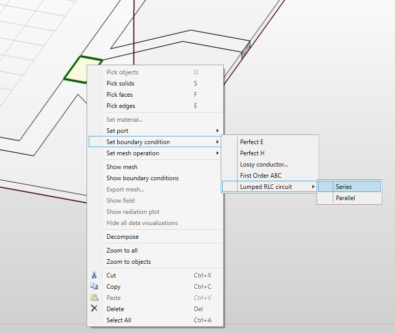
InventSim allows one to define a rectangular 2D surface object as a two-port device that represents a parallel or series RLC circuit. To model an RLC circuit impedance boundary condition is applied. At least one value of R,L,C provided by the user must be non-zero.
To define the 2D rectangle as an RLC element you need to select the object, invoke the context menu (with right-click) and select the option ’Set boundary condition -> Lumped RLC circuit -> Series Parallel.’ (Fig.4.1). Then we define which pair of opposite edges are element connectors and define the values of resistance R, inductance L, and capacitance C.
4.5 Absorbing boundary condition
In order to truncate the mesh and simulate the infinite free-space environment needed, for example, in antenna applications, an artificial surface that absorbs radiated field should be used. With InventSim, you can introduce an absorbing boundary condition (ABC) that absorbs the incident waves and minimizes reflections from the surface [2]:
\(\seteqnumber{0}{}{9}\)\begin{equation} \hat {n} \times (\nabla \times \textbf {E}) + j k_0 \hat {n} \times ( \hat {n} \times \textbf {E}) = 0 \end{equation}
This type of absorbing boundary condition is most efficient when a plane wave direction is perpendicular to the surface and, in the case of incident, at an angle large enough to the surface so that a significant reflection can be observed. In most cases, the recommended minimum distance between the surface and the source of radiation is one-half wavelength. The advantage of using such absorbing boundary condition is the simplicity of its definition on one or several surfaces, including non-planar ones.
When simulating radiating elements, we utilize the fields gathered from radiation boundaries to assess key radiation parameters such as pattern, radiation efficiency, or gain.
4.6 Symmetry planes
The symmetry of the structure can be exploited to reduce the numerical cost of simulation. It can be done by simply cutting the structure in the symmetry plane and enforcing a proper boundary condition.
In InventSim, both PEC and PMC walls can be used as the symmetry planes. The choice to use the symmetry plane and which kind (PEC, PMC) is dependent on the structure and the properties of electromagnetic field solution within the structure, and it requires proper knowledge and experience of the user. In general we:
-
• use PEC where the magnetic field is symmetric and electric field is asymmetric.
-
• use PMC where the electric field is symmetric and magnetic field is asymmetric.
4.6.1 Example
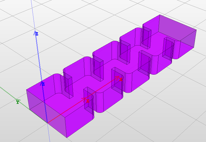
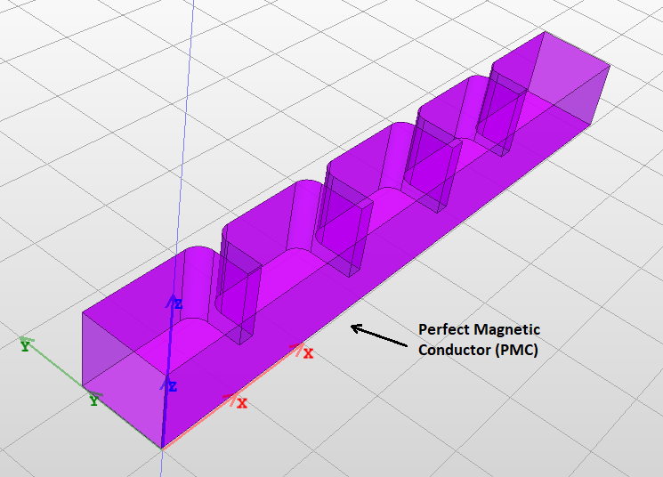
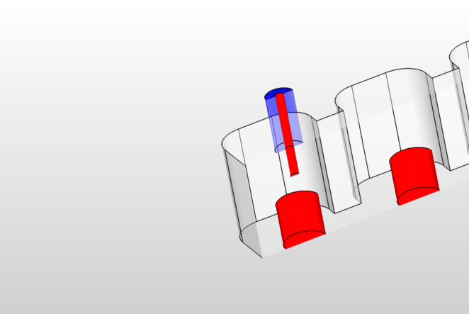
The application of symmetry planes can be shown in an example of the H-plane waveguide filter simulation. The 3D view of the structure is shown in Fig. 4.2. One can notice that the structure is symmetric with respect to XZ-plane. Only \(TE_{n0}\) modes (with \(n=1,3,5...\)) are excited within the structure. The electric field is symmetric along the symmetry plane and all modes have a maximum of the electric field (and zero magnetic field) in the symmetry plane. Therefore, instead of simulating the whole structure, you can cut a half of it (Fig.4.3), and define the surface on symmetry plane as a perfect magnetic conductor.
The port can be added now - InventSim will calculate the mode templates that take the symmetry into account. In result, you can reduce the problem size by half while preserving the accuracy of the simulation at the same time.
4.7 Boundary conditions visualization
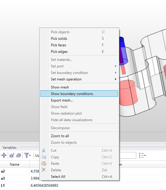
When working with complex structures where many boundary conditions are set, it is often hard to confirm whether the resulting simulation domain is set correctly. A convenient tool for checking boundary conditions is boundary conditions visualization which displays boundary condition types in the Scene view. When the view is enabled each face of structure is assigned a color based on boundary condition type allowing them to be easily distinguished from each other. The colors are described in a legend displayed in the top left corner of the Scene. To add a boundary conditions visualization select "Show boundary conditions" from the Scene context menu (Fig.4.4).
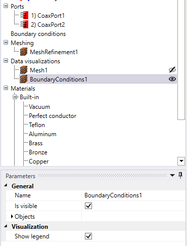
Once added the visualization will be visible in the project tree (Fig.4.5). Boundary visualization parameters are:
-
• Name: the name of the visualization.
-
• Is visible: indicates whether visualization is displayed or not.
-
• Objects: not used.
-
• Show legend: indicates whether visualization legend is displayed or not.

Boundary conditions view displays faces in opaque colors which means most of structure is obstructed from the view. In order to view entire structure cut view can be enabled as described in Section 3.1.1.
5 Material definitions
A core part of electromagnetic field simulation is the definition of electric properties of materials for all 3D objects defined in the structure. In InventSim, you can use several different types of materials, i.e.:
-
• Isotropic, frequency independent dielectric
-
– Lossless
-
– Lossy, with provided loss tangent
-
-
• Isotropic, frequency-dependent dielectric
-
– Debye model
-
-
• Bulk conductors with provided conductivity \(\sigma \)
-
• Gyromagnetic materials described with Polder tensor
The list of materials is shown in the project tree window, Fig.5.1.
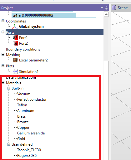
There are several predefined materials available:
-
• Vacuum
-
• Perfect conductor
-
• Teflon
-
• Aluminum
-
• Brass
-
• Bronze
-
• Copper
-
• Gallium arsenide
-
• Gold
Please note that there are two ways to handle PEC objects in your simulation:
-
• Define the material of the 3D object as PEC. When you do this, the software includes the object in the simulation as a 3D volume, and it discretizes the object with a mesh. Since PEC is impenetrable by EM fields, meshing of PEC objects may be unnecessary.
-
• Alternatively, you can choose to remove the PEC object from your model. By default, the boundary condition on the outer surfaces of your model is set to PEC. This means that any surface where you removed the PEC object will automatically be treated as if it’s a perfect electric conductor. This approach is considered more efficient because it avoids generating a 3D mesh for PEC volumes. Instead, it simplifies the simulation by assuming that the outer surfaces of the removed object act as if they were PEC.
5.1 Adding materials
To add a new, user-defined material, select "Materials" in the project tree, then select "Add" from the context menu. The new material, by default, will have the properties of vacuum. Alternatively, you can use a built-in material as the template for the new material by selecting the built-in material and using Copy/Paste commands. By doing this, the new material will have the properties of the selected built-in material.
5.2 Advanced materials
5.2.1 Bulk conductors
In InventSim, lossy bulk conductors with finite conductivity \(\sigma \) are modeled as lossy dielectric material using a model of dielectric permittivity:
\(\seteqnumber{0}{}{10}\)\begin{equation} \epsilon _r = \epsilon _r' - \frac {j\sigma }{\omega \epsilon _0} \end{equation}
In general, metals are described as having an effective permittivity with real relative permittivity \(\epsilon _r'\) equal to one.
To define the material as a lossy conductor, you need to define its finite conductivity. Please note that material losses can be defined either with non-zero dielectric loss tangent (frequency independent lossy dielectric material) or non-zero, finite conductivity (frequency dependent bulk conductor):
-
• When you assign a material with finite conductivity to a 3D solid, the solid is treated as a volumetric conductor. In this scenario, electromagnetic waves can penetrate the volume. To represent this, the volume is divided into small tetrahedral elements (tetrahedral mesh), and the material is modeled with a frequency-dependent approach. It’s important to note that simulating such configurations requires a significant increase in computational effort. Another consequence of defining volumetric conductors in your project is that you cannot use the ’Fast Frequency Sweep’ option. Instead, you must choose either the ’Interpolating Sweep’ or the ’Discrete Sweep’ method for your simulations.
-
• Usually, to model the lossy conductor, it is enough to define a proper boundary condition on the surface of the volume. Please refer to section 4.3 for more details.
5.2.2 Debye dielectric
In many medical applications, a Debye model of dielectric is used to model the biological tissue and possible hazards. In InventSim, a basic, single-pole Debye dielectric is defined by complex frequency dependent permittivity:
\(\seteqnumber{0}{}{11}\)\begin{equation} \epsilon _r(\omega ) = \epsilon _{inf} + \frac {\epsilon _{dc} - \epsilon _{inf} }{1+\omega \tau } \end{equation}
Single pole Debye dielectric model is defined with three double values: \(\epsilon _{inf}\), \(\epsilon _{dc}\) and time constant \(\tau \).
5.2.3 Gyromagnetic
A wide class of microwave devices uses a ferrite materials to achieve non-reciprocal response. Many of them use saturated ferrite, which magnetic permeability is described by Polder tensor:
\(\seteqnumber{0}{}{12}\)\begin{equation} \mu = \mu _0 \left [ \begin{array}{ccc} 1+\chi _{xx} & \chi _{xy} & 0 \\ \chi _{yx} & 1+\chi {yy} & 0 \\ 0 & 0 & 1 \end {array} \right ] \end{equation}
where:
\(\seteqnumber{0}{}{13}\)\begin{equation} \chi _{xx} = \chi _{yy} = \chi ' - j\chi " \end{equation}
\(\seteqnumber{0}{}{14}\)\begin{equation} \chi _{xy} = -\chi _{yx} = j(K' - jK") \\ \end{equation}
\(\seteqnumber{0}{}{15}\)\begin{equation} \chi ' = \frac {\omega _0 \omega _m (\omega _0^2 - \omega ^2) + \omega _m \omega _0 \omega ^2 \alpha ^2 }{(\omega _0^2 - \omega ^2(1+\alpha ^2))^2 + 4\omega _0^2 \omega ^2 \alpha ^2} \end{equation}
\(\seteqnumber{0}{}{16}\)\begin{equation} \chi " = \frac {\omega \omega _m \alpha (\omega _0^2 + \omega ^2 (1+\alpha ^2 ))^2} {(\omega _0^2 - \omega ^2(1+\alpha ^2))^2 + 4\omega _0^2 \omega ^2 \alpha ^2} \end{equation}
\(\seteqnumber{0}{}{17}\)\begin{equation} K' = \frac {\omega _0 \omega _m (\omega _0^2 - \omega ^2(1+\alpha ^2))^2 }{(\omega _0^2 - \omega ^2(1+\alpha ^2))^2 + 4\omega _0^2 \omega ^2 \alpha ^2} \end{equation}
\(\seteqnumber{0}{}{18}\)\begin{equation} K" = \frac {2 \omega ^2 \omega _0 \omega _m \alpha }{(\omega _0^2 - \omega ^2(1+\alpha ^2))^2 + 4\omega _0^2 \omega ^2 \alpha ^2} \end{equation}
\(\seteqnumber{0}{}{19}\)\begin{equation} \omega _m = \mu _0 \gamma M_s \end{equation}
\(\seteqnumber{0}{}{20}\)\begin{equation} \omega _0 = \mu _0 \gamma H_0 \end{equation}
\(\seteqnumber{0}{}{21}\)\begin{equation} \Delta H = \frac {2 \alpha \omega }{\mu _0 \gamma } \end{equation}
where \(\gamma \) is a gyromagnetic ratio, \(\omega _0\) is the free precession angular velocity (Larmor frequency),\(H_0\) is the static magnetic field strength, \(M_s\) is the saturation magnetization of a ferrite material and \(\Delta H\) is the linewidth of the gyromagnetic resonance corresponding to ferrite losses. In most cases, we use \(\gamma = 1.760859 \cdot 10^{11}\) As/kg, but you can modify this value with user defined Lande g-factor \(L_u\) as
\(\seteqnumber{0}{}{22}\)\begin{equation} \gamma _{user} = \gamma \cdot \frac {L_{u} }{L_0} \end{equation}
where \(L_0\) = 2.002319.
Material properties are defined by saturation magnetization \(M_s\) [A/m], DC magnetic field \(H_0\) [A/m], linewidth \(\Delta H\), Lande g-factor \(L_u\) and the local coordinate system that defines the magnetization direction along Z-axis.
5.3 Influence on simulation time and memory requirements
If a medium used in the simulation is lossy, then the solver uses complex arithmetic to solve the problem. Therefore, any simulation with dielectric/conductor losses and/or absorbing boundary conditions will demand around twice as much memory as the simulation with lossless structures. For the same reason, the simulation will take longer to complete.
If any material in the project is defined as a tensor or a gyromagnetic, the computations are conducted on unsymmetrical matrices, which doubles the memory required to perform a simulation.
6 Adding ports
InventSim supports a few types of wave ports. Depending on the structure, you should select the port type that fits the mode type which propagates in the transmission line of a provided cross-section. To add a port to the structure, you need to select the surface that will constitute the port (to pick the surface, enable "Pick face" mode with the shortcut key "F"), then click the right mouse button and select "Set port -> ..." (Fig. 6.1) Port type cannot be changed after the port has been assigned. In order to change the type, delete the port and assign it again with a different type. To delete a port, select it in the project tree and select "Delete" from the context menu.
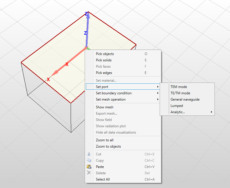
If the face to which a port is assigned to is deleted (either by explicit deletion or as a result of structure change), the port will be deleted automatically.
Depending on the simulation frequency, the transmission line that is defined as a port surface can guide more than one mode (there is more than one mode above cutoff). In this case, you should define the port as a multi-mode port (the option is available for a general port and TE/TM port).
The wave port can be assigned on any planar surface defined by the user, but few restrictions are enforced:
-
• The solver does not support open (radiating) transmission lines on the ports. Only closed transmission lines are supported at the moment. If a radiating boundary condition is defined at port edge, it will be neglected and transformed to a PEC on the stage of port analysis.
-
• TEM, TE/TM and general wave ports can be defined only at the outer surfaces of the domain. Lumped ports can also be defined as internal ports.
-
• The wave port should be placed at a moderate distance from any discontinuity of the transmission line. Please note that the port terminates (absorbs) only the modes that were evaluated at this port. Any other mode that propagates from discontinuity to the port will be reflected back to the structure.
-
• In general, all wave ports are normalized to the wave impedance of the line. You can re-normalize the calculated scattering parameters to characteristic impedance of the line only in the case of lumped ports.
-
• When the solver searches for modes propagating in the ports, it handles the transmission line as a lossless one. If any lossy medium is defined in the port, then the solution found by the solver might be slightly mismatched with a lossy line. An additional reflection on the connection of the lossless and lossy lines will be introduced.
-
• The port must be defined on the wall of a 3D object. Surfaces placed arbitrarily in space are not allowed.
-
• The port should enclose all the conductors needed to properly solve the excitation mode field pattern.
6.1 TEM mode ports
This type of a port can be used to simulate a homogeneous two conductor line, i.e. a coaxial line. The coaxial cable is one of the most common transmission lines used in high frequency and microwave devices. It is a two-conductor line of a cylindrical cross-section, in which an inner rod and outer shielding conductor are placed concentric on the same axis and it is usually separated with dielectric material. In this type of transmission line, the fundamental propagating mode is TEM mode with zero cutoff frequency.
In order to find the proper TEM mode template, InventSim numerically solves the Laplace equation defined by a provided port cross-section
\(\seteqnumber{0}{}{23}\)\begin{equation} \nabla ^2 \phi = 0 \end{equation}
assuming 1V potential difference between two conductors. In this case, only a single mode propagation is available. In order to handle higher order modes, you should use a general port.
6.2 TE/TM mode port
Transverse electric (TE) and transverse magnetic (TM) are modes with non-zero cutoff that are propagating in homogeneous, single-conductor, closed transmission lines. Some examples are rectangular, circular or elliptic waveguides. To solve the TE mode template \(\textbf {E}_t\) the vector wave equation is solved:
\(\seteqnumber{0}{}{24}\)\begin{equation} \nabla _t \times ( \mu _r^{-1} \nabla _t \times \textbf {E}_t ) - k_c^2 \epsilon _r \textbf {E}_t = 0 \end{equation}
and for TM modes:
\(\seteqnumber{0}{}{25}\)\begin{equation} \nabla _t \times ( \epsilon _r^{-1} \nabla _t \times \textbf {H}_t ) - k_c^2 \mu _r \textbf {H}_t = 0 \end{equation}
where \(k_c\) is the cutoff frequency of the mode.
This type of a port supports multimodal regime and the number of modes is specified with cutoff frequency \(k_c\). If you introduce the non-zero cutoff frequency at the port, then the solver searches for all modes that are propagating up to a provided cutoff frequency \(f_c\). Please note that you will get a multimodal (generalized) scattering matrix as the simulation result.
Efficiency notice: TE/TM ports are solved using a dense matrix eigensolver, which can be computationally intensive for very dense meshes at the ports. In this case, it is recommended to use general ports that use sparse matrix computations.
6.2.1 Degenerate TE/TM modes
In some, special transmission lines, (i.e. circular or square waveguide) a pair of modes with the same cutoff can propagate along the line with the same propagation constant, but different polarization. It is very difficult to properly control the polarization of both numerical solutions unless the analytic solutions are known and used. At the moment, InventSim might produce inaccurate results for ports with degenerate mode propagation. One can overcome this by slightly changing the cross-section. As an example: instead of square waveguide with sidewall dimension \(a=20mm\), simulate rectangular waveguide with dimensions \(a=20mm\) and \(b=20.01mm\).
6.3 General ports
This type of a port is the most robust one and it can be applied to transmission lines with any cross-section, including waveguides loaded with inhomogeneous dielectrics. The most common application of this port would be a microstrip line, a co-planar waveguide or a partially filled rectangular waveguide. To solve the mode template at the port, a three-component vector field formulation is implemented, which solves the equations:
\(\seteqnumber{0}{}{26}\)\begin{equation} \textbf {E} = \textbf {E}_t + \hat {n} E_z \end{equation}
\(\seteqnumber{0}{}{27}\)\begin{equation} \nabla _t \times ( \mu _r^{-1} \nabla _t \times \textbf {E}_t ) - \mu _r^{-1}(j \beta \nabla _t E_z - \beta ^2 \textbf {E}_t) = k_0^2 \epsilon _r \textbf {E}_t \end{equation}
\(\seteqnumber{0}{}{28}\)\begin{equation} -\mu _r^{-1} [ \nabla _t \cdot ( \nabla _t E_z + j \beta \textbf {E}_t ) ] = k_0^2 \epsilon _r E_z \end{equation}
for a provided frequency \(k_0\).
General ports can also handle multi-modal propagation. In port options, you can specify the number of modes that should be taken into account during the simulation (Fig. 6.2). Initial value equal to zero means that just a fundamental (lowest cutoff) mode is found. For example, if you simulate coupled microstrip lines that consist of three conductors, then two modes should be defined at the port.
You can also add a coordinate system to the port with (
 ) icon. If one is added, the solver will try to align the sign of the electric field component of mode template with Z-axis of coordinate system defined at the port.
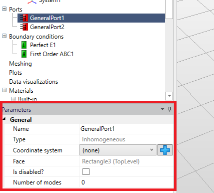
In these types of ports, a mode template has to be found on each frequency and the associated numerical cost is the highest when compared to TEM or TE/TM modes. In that respect, the TEM ports or TE/TM ports should be used, if possible, to reduce the computational cost involved.
6.3.1 Microstrip and CPW ports
Both CPW and microstrip lines are in, general, in-homogeneous cross-section lines. To properly simulate the devices with those line types, general ports should be used. Additionally, since the CPW line is a three conductor line, it guides two different modes with zero cutoff frequency (even and odd) (Fig.6.3). In order to properly solve the CPW line, both modes should be taken into account during the simulation by setting the number of modes in the port as two. Then you can identify the mode you are mainly interested in (usually the even mode).
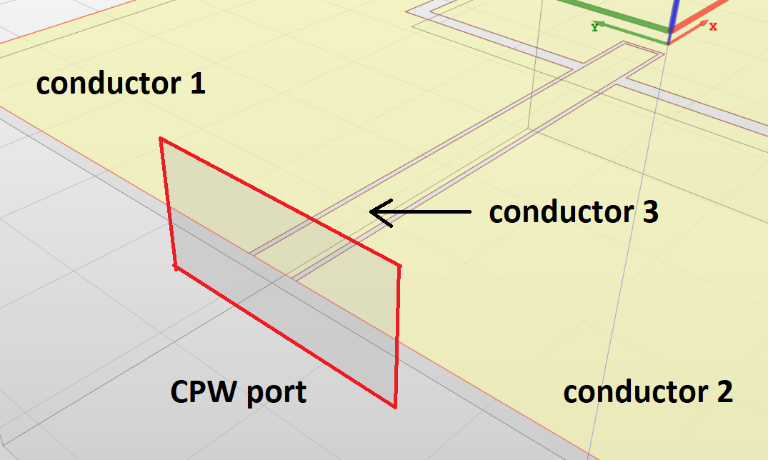
6.4 Lumped ports
Lumped ports are the only ports that can be placed inside of the domain and assume that the port is much smaller compared to the wavelength. The surface on which the port is defined must cover at least two conductors. To define a lumped port, you need to also define a voltage plan - i.e. assign voltage (0V or 1V) for each conductor. Then, during the simulation, the solver computes the currents that flow between the conductors and calculates the impedance parameters.
Please note that in InventSim lumped ports should be defined on homogeneous dielectric areas!
6.4.1 Adding lumped ports
To show an example of the lumped port definition, let us look at the microstrip line structure shown in Fig. 6.4. The structure consists of two box objects representing the dielectric substrate layer and the air above it. It also consists of a 2D rectangular object that is a PEC strip. To excite the structure with lumped ports, you need to define the port area first. In this case, it is a small rectangular area between the strip and the ground-plane.
Draw a 2D rectangle that covers this area, as shown in Fig. 6.5. Then modify the default boundary condition on the wall from PEC to PMC (otherwise the strip would be shorted to the ground, Fig. 6.6. In the next step, select the 2D rectangle object and select "Set port -> Lumped" (Fig. 6.7 from the context menu.
A new lumped port will be added. Select this port, go to the properties window and add an excitation mode template (using
icon). InventSim will process the port area to find the conductors defined at the port. Once that is done, the conductors will be shown in the 3D view and marked with labels (Fig. 6.8). With the voltage plan options, you can define the value of voltage for each conductor - in this case it is 0V for the ground-plane and 1V for the conducting strip.
Optionally, you can define the reference impedance (default is 50 Ohm) used to re-normalize calculated scattering parameters.
The user can optionally apply port calibration, i.e. technique that removes the port discontinuity from the numerical simulations. This might influence the simulation results in high frequency regime.
To properly model lumped ports (defined on 2D objects), InventSim requires them to be drawn on the surfaces or walls associated with 3D objects. If the lumped port is drawn inside of the volume, an auxiliary 3D element should be drawn and the port should be defined on the surface of this 3D object.
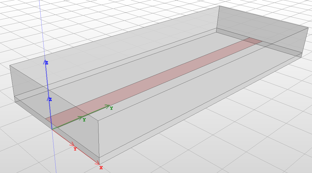
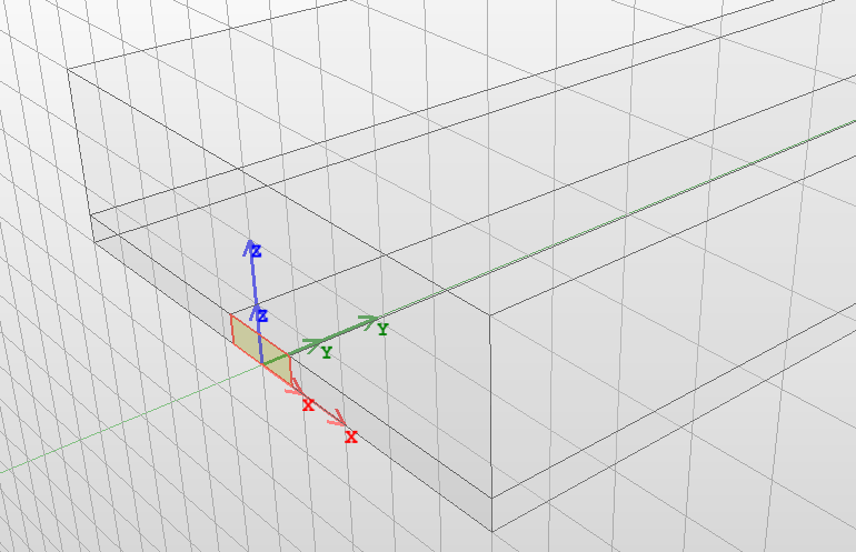
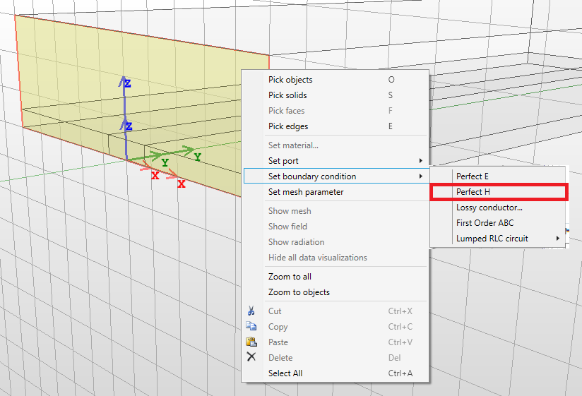
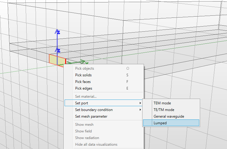
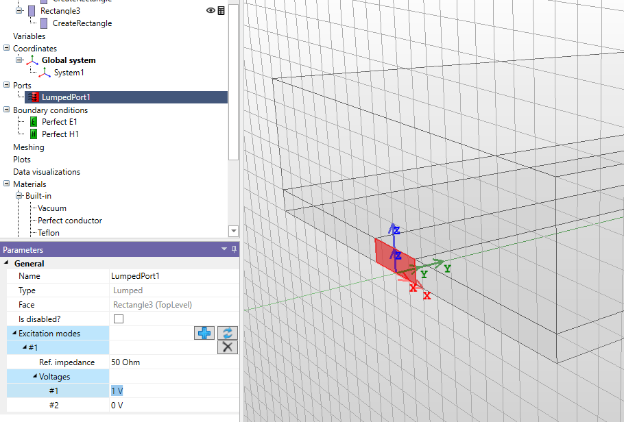
6.5 Analytic ports
Analytic ports provide a way to specify the excitation within the port plane using analytical solutions for modes propagating in strictly rectangular or circular waveguides. This capability enables precise control over the excitation’s phase and ensures accurate computation of the resulting scattering parameters.
Important Note: When dealing with square waveguide or circular waveguide ports, it’s crucial to understand that numerical solutions for mode field templates cannot offer exact mode polarization definitions.
-
• In the case of square waveguides, the numerical solution describes a linear combination of the \(TE_{10}\) and \(TE_{01}\) modes.
-
• or circular waveguides, the degenerate solutions for \(TE_{mn}\) or \(TM_{mn}\) waveguide modes with \(m \ne 0\) are indistinguishable in the solution.
Only the use of analytic field templates allows the user to properly define excitation in this scenario, and we strongly recommend employing analytic modal field solutions.
To define an analytic mode template, the user must provide additional information regarding the mode type (TE/TM) and the mode indices (m, n). Modes can be added with port’s property panel. The modes align with the local coordinate system defined at the port, with the "z" direction indicating the propagation direction. User can add more than one mode to the port, enabling the calculation of multimodal, generalized scattering matrix of the component.
7 Meshing options
Mesh generation is a crucial part of every finite element simulation. Its task is to construct a discrete representation of a modeled geometry. In InventSim, we use a tetrahedral grid in order to be able to model complex, arbitrarily shaped geometries.
To generate a mesh, InventSim uses the third party software Netgen [12, 13] that generates good-quality, second-order grids. The mesh influences the accuracy of simulation results in several ways:
-
• The mesh is a discrete representation of original geometry. The meshing process can introduce a discretization error, especially if curved boundaries are present in the structure. In InventSim, to achieve a better representation of curved shapes, we use a second order mesh, where the element edges are second order curves (Fig. 7.1).
-
• In order to properly model the field behavior, the mesh needs to be adequately fine. In general, it is recommended to set the initial, vglobal maximum mesh edge length as \(\frac {\lambda _{min}}{5}\), where \(\lambda _{min}\) is the wavelength at the maximum simulation frequency. However, in regions that exhibit strong field variation, you may need to refine the mesh. In InventSim, you can use adaptive mesh refinement to improve the accuracy of the results.
-
• Poor-quality, needle-like or nearly flat tetrahedral elements with high aspect ratio would result in deterioration of main matrix conditioning number. This might cause problems during the solution phase, especially if iterative solvers are used.
The meshing options can be found in the "Simulation" tab on the right side of the main GUI window (Fig. 7.3). The window is divided to two sections: global mesh and adaptive meshing options.

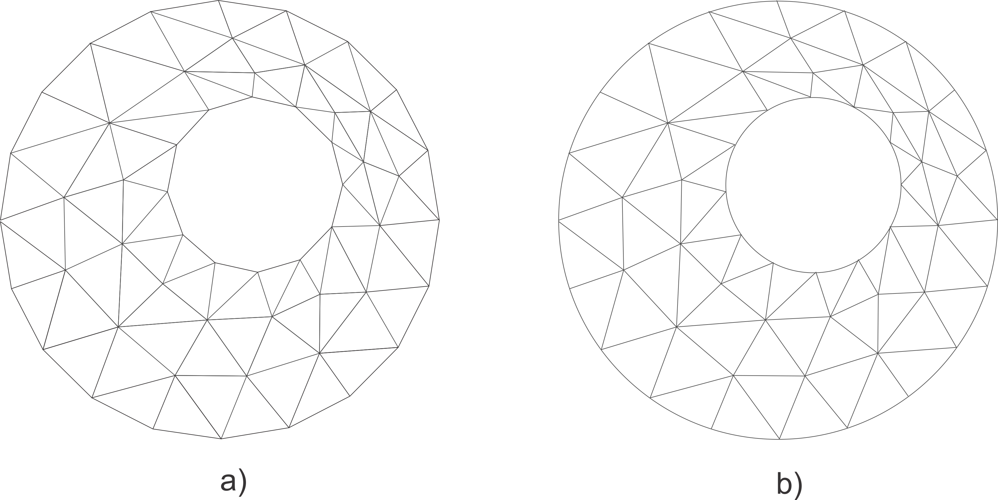

7.1 Global mesh settings
The process of meshing creates a tetrahedral volume mesh and a triangular surface mesh, based on the geometrical model of the structure. A single mesh cell size as well as the global distribution of cell sizes are determined by several factors.
Default behavior of the meshing is controlled by global options located in the "Global parameters" section of the "Mesh" tab. These options include:
-
• Maximum mesh size - the maximum edge length in the mesh (global). This setting determines uniform refinement of the mesh.
-
• Segments per radius - defines the number of sections into which the curved edges will be divided. This determines how well the round edges will be approximated.
-
• Segments per edge - defines the number of sections into which the straight edges will be divided.
-
• Grading - specifies the amount of variation in the size of adjacent cells. Normal is the default value, which allows a certain degree of local mesh refinement. Low setting value results in a more uniform mesh, while High setting generates highly non-uniform mesh.
7.2 Adaptive meshing
A typical structure consists of regions where the mesh needs to be refined, while at the same time there are other regions where the mesh can be coarse without sacrificing the accuracy. It is difficult to predict the areas where the finer mesh is required, therefore the adaptive meshing procedure should be used. The repeating procedure refines the mesh locally in order to improve the accuracy of the results.
The accuracy is tested at a set of frequency points by comparing the magnitudes of scattering parameters calculated at those points. The procedure stops when a specified number of consecutive simulations report the results differing by less than a specified value.
The adaptive meshing is set up in the "Mesh" tab of the "Simulation" panel. The procedure can be switched on and off by selecting "Use adaptive meshing" checkbox. The frequencies at which the accuracy is tested are defined in a fashion similar to setting the simulation frequencies (please see "Frequency sweep simulation" chapter for details). The main parameters of the adaptive meshing are:
-
• Accuracy - the maximum difference between the magnitudes of scattering parameters.
-
• Mesh size increase - the fraction of the mesh vertices that will be designated for refinement. The higher the value, the greater the problem size in consecutive iterations.
-
• Maximum iterations - the total number of iterations.
-
• Converged iterations - the number of iteration that allow the error to be smaller than "Accuracy" after which the adaptive meshing will converge.
In practice, your experience and knowledge about field solutions predicted within the structure might be used to make the initial mesh as good as possible. This would limit the number of adaptive mesh iterations and therefore reduce the simulation time. To refine the mesh locally, you can use "Local" mesh parameters.
7.2.1 Enabling adaptive mesh frequencies
The adaptive mesh refinement is disabled by default. To enable it, you need to click the "Adaptive meshing" checkbox and add at least one (possibly more) frequency point. The convergence of the adaptive mesh refinement will be tested at this point(s). To add a frequency, please click the right mouse button on the "Frequencies" window to use the context menu. Then select "Add" and define the start, stop and a number of frequency points - usually this will be done on just one or two points to reduce the simulation time. Here are the recommendations:
-
• In non-resonant, transmission-line structures define the frequency as the highest frequency of simulation,
-
• In resonant structures, like filters, define the frequency close to the passband or within the passband, since the field variations are at the highest close to the resonance,
-
• If a structure has multiple resonances with different modes or located in a different part of the domain, then you can define more than one frequency close to the resonant frequencies. It is done to properly model field variations at the resonance.
7.2.2 Example
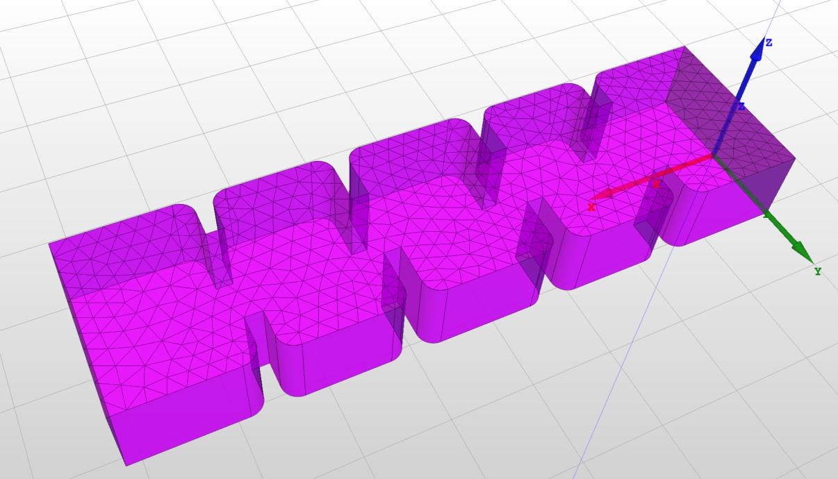
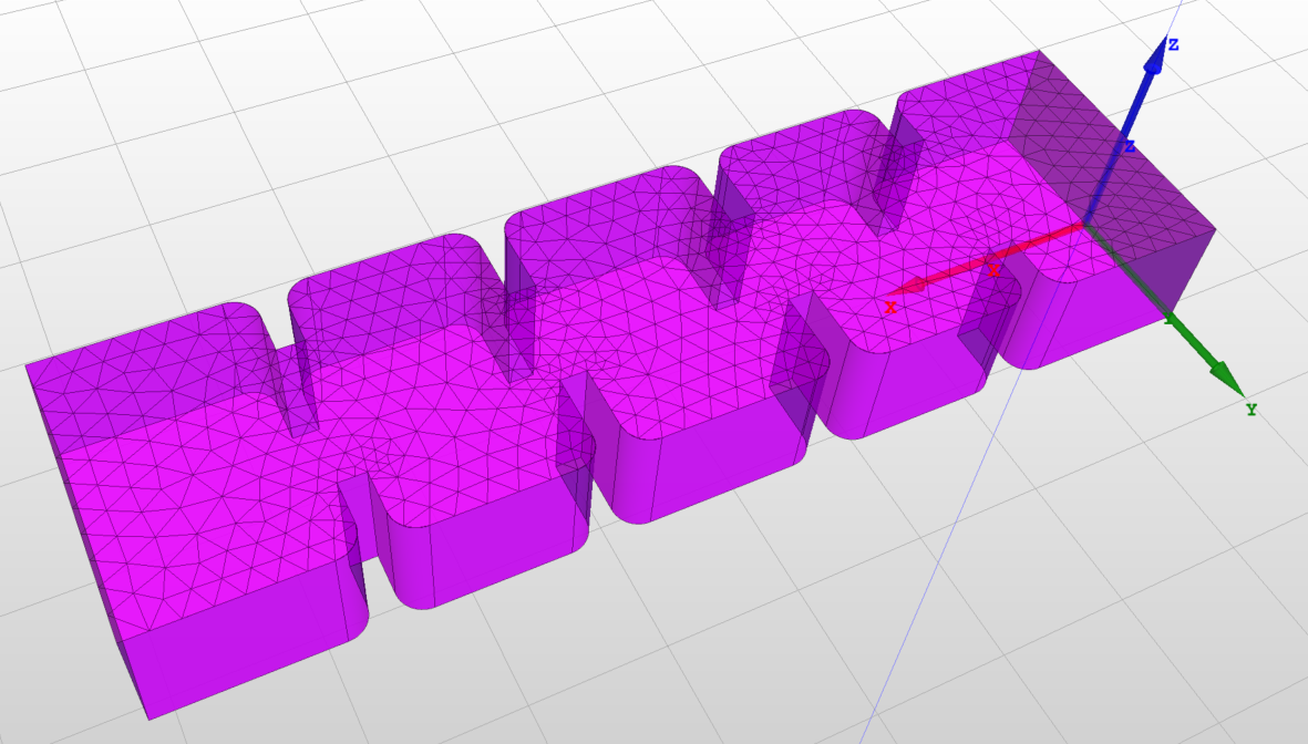
Fig. 7.4 presents an example of an application of adaptive mesh refinement using a simple, H-plane waveguide filer. When comparing the uniform mesh with the adaptively refined mesh, it is noticeable that the adaptive mesh refinement algorithms implemented in InventSim allow you to generate a mesh that can represent the fields in the structure in a positive way: the most important areas that have a high field variation will have a much smaller mesh size.
7.3 Mesh refinements
Another tool that allows control of mesh behavior is Mesh refinements. It allows to restrict mesh cell size in selected regions of space in order to override global mesh settings. It can be used either in conjunction with Adaptive meshing or instead of it, depending on the application and the user’s understanding of the structure field behavior.
The local meshing behavior can be controlled by introducing one or more Mesh refinements to the project. Each of the refinement defines a set of rules on how to restrict mesh cell size. These rules, along with global mesh parameters, are passed to the mesher during meshing phase. Each rule consists of three conceptual parts:
-
1. Objects - in conjunction with the next part, defines region(s) in 3D space where mesh size would be restricted. SimObjects are used for the user’s convenience to define regions in space.
-
2. Relation - defines which topological part(s) of Objects should be used to determine region(s) of 3D space. The possible choices are listed below and its results depend on SimObject type.
-
• Inside, on surface and edges
-
• On surface and edges
-
• On edges
[parsep=1pt, topsep=1pt]
-
-
3. Maximum length - defines the maximum size of mesh cell in length units.
[parsep=2pt]
To add a mesh refinement, select the desired solid or a face, open context menu and select "Set mesh operation->Refinement" (Fig. 7.5). The new mesh refinement will be added to the project tree with the following list of parameters:
-
• Name: the name of the refinement.
-
• Is enabled: indicates whether the refinement is enabled or not.
-
• Maximum length: maximum mesh cell size.
-
• Relation: sets how the refinement will be applied to the selected objects.
-
• Objects: list of objects on which the refinement is set.
[itemsep=2pt, parsep=2pt]
To delete the mesh parameter, first select it in the project tree and then choose "Delete" from the context menu.
If multiple mesh refinements are defined on the same region(s) of space the most restricting parameter will be in effect i.e. the one with the smallest "Maximum length" value. No error nor warning will be shown.
Mesh refinements can also be set on SimObjects which have "Calculate" flag off. Using such a feature user can define an arbitrary region in space which exhibit a desired meshing behavior but does not introduce any geometrical entities into the simulation domain.
7.3.1 An Example
In this example, the structure consists of a simple box sized 5mm x 8 mm x 10mm. The box is discretized with a uniform mesh that has an edge length equal to 3mm, as shown in Fig. 7.5. To refine the mesh on the upper surface, you need to select this surface, then select the "Set mesh parameter" option in the context menu. A new position will appear on the project tree. It is added in the "Meshing" section - it allows you to enter the maximum edge length. If you input 0.8mm, you will get a non-uniform mesh as shown in Fig. 7.5.
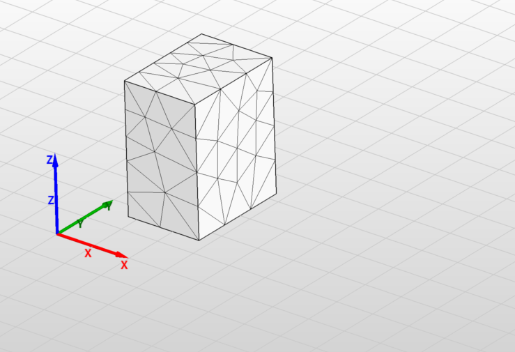
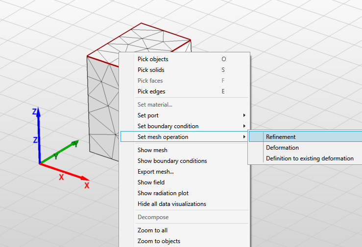

7.4 Mesh morphing
The simulation with the finite element method requires a discrete representation of the model using a mesh. The mesh has to be generated every time the model changes - i.e. the geometrical structure dimensions are modified. Common practice in most simulation software tools in this case is to generate the mesh from scratch. Even if the geometry change was comparably small and localized in a small part of the model, the mesh is re-generated for whole structure. Such an approach has several disadvantages [28]:
-
• Mesh generation is a time consuming procedure, especially when adaptive mesh refinement is involved.
-
• Re-meshing noise can be observed, this means that the model geometry change is continuous, while the change of model response is not continuous.
-
• During the solution phase, all data from the previous simulation is lost and the solver starts from scratch.
In InventSim, mesh morphing algorithms are implemented to eliminate those issues. Mesh morphing allows you to modify the existing mesh and move mesh nodes to fit the modified model. As a result, the mesh topology does not change: what changes is only the locations of mesh nodes.
In general, InventSim can morph the mesh of arbitrary, user-defined 3D geometry. There is a restriction though: the modified geometry should have the same topology as the original - i.e. number of the faces and the edges and their connections should remain the same.
Mesh morphing can be used during optimization and tuning. It can also be invoked by the COM interface.
7.4.1 Using COM to morph a mesh
InventSim can be used to perform mesh morphing of a 3D model without further simulation. In order to generate a morphed mesh for a modified geometry, please follow these steps:
-
• Load and simulate the project to generate the mesh for initial geometry. The 3D model should be parameterized with variables - only optimization variables can be changed during mesh morphing. Important: the current mesh must correspond with actual model geometry!
-
• Connect to the COM server, for example using Matlab/Octave, as shown in Section "COM Interface".
-
• Load the set of current values of optimization variables using the COM function:
x0 = App.ActiveProject.Variables.GetOptimizableVariableValues(); -
• Provide the vector of modified variables x1.
-
• Obtain reference mesh:
refMesh = app.ActiveProject.Simulation.GetMesh(); -
• Execute mesh morphing using COM method:
morphedMesh = App.ActiveProject.Simulation.GetMorphedMesh(refMesh, x0, x1, 0);
Modified mesh is returned by the method. -
• Optionally, restore the original values of variables with this method:
App.ActiveProject.Variables.SetOptimizableVariableValues(x0);
To repeat the simulation using the morphed mesh, set OverrideMesh property of Simulation with the reference to the morphed mesh and start simulation:
App.ActiveProject.Simulation.OverrideMesh = morphedMesh;
App.StartSimulation();
7.5 Shape deformations
The use of additive manufacturing (AM) technology (also known as 3D printing) to fabricate high-frequency components has been increasing in popularity in recent years. AM allows for the production of complex 3D structures of almost arbitrary shapes, with user-defined surface curvatures. This flexibility in model complexity is a great advantage over established technologies, as the limitations of conventional techniques such as CNC milling no longer apply. In many cases, AM permits the production of a model that would not be achievable using other manufacturing methods. In this context, AM is a key enabling technology that opens up new possibilities to RF & microwave engineers.
However, in order to take advantage of this design flexibility, the limitations of the CAD tools used in the industry need to be overcome. These limitations stem from the fact that virtually all CAD software used for high-frequency electronic design relies on the constructive solid geometry (CSG) approach. CSG is the prevailing paradigm for the 3D modeling of electromagnetic structures. It is based on using a set of simple, predefined geometrical primitives—such as boxes, cylinders, and cones—and applying to them Boolean operations, such as union, subtraction, and intersection, or shape modifications with edge filleting or chamfering. Alternatively, arbitrarily shaped surfaces based on parametric, equation-based objects can be used, but this is cumbersome and difficult to use. The design of more complex geometrical models—such as those with unconventional twisted or bent shapes—is very challenging in this approach. For decades, the CSG approach has been regarded as satisfactory, as design was limited by the available manufacturing technologies, such as CNC milling. This has now changed with the widespread availability of repeatable and accurate 3D printing.
Therefore, to enable the design of microwave components with truly arbitrary shapes, the solution available in InventSim is to empower CSG-based 3D solid modeling tools with a free-form shape deformation technique.
Shape deformation can be treated as an additional step in the design process. It can be performed on objects created initially with CSG. The basic principle of shape deformation is to define a set of points around the object that will control the deforming operation. The deformation is then begun by shifting some of these control points to certain new coordinates, and a vector displacement field is constructed using these displacements. The original structure is then mapped according to this smooth displacement function. The deforming operation can be performed on 3D objects represented by a surface or volume mesh. In InventSim, we consider a tetrahedral mesh used in 3D FEM.
7.5.1 Shape deformation with RBFs
Shape deformation feature in InventSim is implemented using an interpolation scheme based on radial basis functions (RBF), as reported in [29, 30, 31, 32]. In general, a RBF is a real-valued function \(\varphi \) whose value is only determined by the distance from the origin, so that \(\varphi (\boldsymbol {x}) = \hat {\varphi }(\| \boldsymbol {x} \|)\). The principle of the reshaping operation is represented in general by a mapping function \(\mathcal {D}\):
\(\seteqnumber{0}{}{29}\)\begin{equation} \begin{split} \mathcal {D}(\boldsymbol {x}) : \mathbb {R}^3 \rightarrow \mathbb {R}^3 \\ \boldsymbol {x} \mapsto \mathcal {D}(\boldsymbol {x}) = \boldsymbol {x} + \boldsymbol {d}(\boldsymbol {x}) \end {split} \end{equation}
In this notation, \(\boldsymbol {d}(\boldsymbol {x})\) can be interpreted as the deformation field applied to the 3D model. In the case of RBF-based deformation, this takes the following form:
\(\seteqnumber{0}{}{30}\)\begin{equation} \boldsymbol {d}(\boldsymbol {x}) = \sum _{i=1}^{{N}} \boldsymbol {\gamma _i} \varphi (\| \boldsymbol {x} - \boldsymbol {x_{i}} \|) + p(\boldsymbol {x}) \end{equation}
where \(N\) is the number of control points defining the deformation, \(\boldsymbol {\gamma _i}\) are the weights corresponding to the radial basis functions \(\varphi \) defined at the positions of the control points \(\boldsymbol {x}_i\) (in 3D \(\boldsymbol {x_i} \in \mathbb {R}^3, \boldsymbol {x_i} = [x_i,y_i,z_i] \)), and \(p(\boldsymbol {x})\) is a low-order polynomial (optional).
To perform the deformation, the mapping operation \(\mathcal {D}\) needs to be specified. The first step is to define a set of \(N\) control points and their displacements, which indicate the direction and value of the offset. Next, a certain type of RBF with its parameters (e.g., radius, exponent) is selected: the choice of basis function affects the manner in which the mesh points are interpolated to match the new positions of the control points.
There are many different RBFs commonly used for multivariate function interpolation, six of which are implemented in InventSim:
-
• Gaussian spline:
\(\seteqnumber{0}{}{31}\)\begin{equation} \varphi (\|\boldsymbol {x}\|) = \exp ({-(\frac {\|\boldsymbol {x}\|}{r}})^2), \end{equation}
-
• multi-quadratic biharmonic spline:
\(\seteqnumber{0}{}{32}\)\begin{equation} \varphi (\|\boldsymbol {x}\|) = \sqrt {\|\boldsymbol {x}\|^2 + r^2}, \end{equation}
-
• inverse multi-quadratic biharmonic spline:
\(\seteqnumber{0}{}{33}\)\begin{equation} \varphi (\|\boldsymbol {x}\|) = \frac {1}{\sqrt {\|\boldsymbol {x}\|^2 + r^2}} \end{equation}
-
• thin plate spline:
\(\seteqnumber{0}{}{34}\)\begin{equation} \varphi (\|\boldsymbol {x}\|) = \left (\frac {\|\boldsymbol {x}\|}{r}\right )^k \ln \frac {\|\boldsymbol {x}\|}{r} \end{equation}
-
• Beckert-Wendland C2 basis:
\(\seteqnumber{0}{}{35}\)\begin{equation} \varphi (\|\boldsymbol {x}\|) = \left ( 1 - \frac {\|\boldsymbol {x}\|}{r}\right )^4 + \left ( 4 \frac {\|\boldsymbol {x}\|}{r} + 1 \right ) \end{equation}
-
• polyharmonic spline:
\(\seteqnumber{0}{}{36}\)\begin{equation} \varphi (\|\boldsymbol {x}\|) = \begin{cases} (\frac {\|\boldsymbol {x}\|}{r})^k \quad & \text {if}~k = 1,3,5,...\\ (\frac {\|\boldsymbol {x}\|}{r})^k \ln (\frac {\|\boldsymbol {x}\|}{r}) \quad & \text {if}~k = 2,4,6,...\\ \end {cases}, \end{equation}
where \(r\) and \(k\) are the radius and power of the RBF, respectively. A linear equation system is then solved to find the unknown weights \(\boldsymbol {\gamma _i}\) given the coordinates of the original and displaced control points [31]. The matrix representation of this equation system is as follows:
\(\seteqnumber{0}{}{37}\)\begin{equation} \boldsymbol {\Phi }\boldsymbol {\gamma } = \boldsymbol {B} \end{equation}
where \(\boldsymbol {\gamma }\) is the weight matrix of dimension \(N\times 3\), corresponding to \(N\) control points defined in a 3D coordinate system. \(\boldsymbol {\Phi }\) is an \(N\times N\) matrix containing RBF values computed for the Euclidean distances between the corresponding control points, \(\boldsymbol {\Phi _{i,j}} = \varphi (\| \boldsymbol {x_{i}} - \boldsymbol {x_{j}} \|)\), and \(\boldsymbol {B}\) is an \(N\times 3\) right-hand side matrix with the new (displaced) coordinates of the control points. The system is dense, symmetric, positive definite, and its conditioning depends on selected RBF and control points distribution. Once the weights are computed, the deformation field \(\boldsymbol {d}(\boldsymbol {x})\) is constructed and can be applied to smoothly move all the mesh points of a 3D object. It can be seen that the mapping function can be easily defined with a limited number of control points, and then applied to create complex 3D objects. The computational cost of the deformation is also not significant, as the size of the linear problem to be solved is usually small.
7.5.2 Example: deformation of a rectangular waveguide
To illustrate the operation of this framework, a simple example of creating a smooth-profile rectangular waveguide filter is presented. First, a basic structure is created using constructive solid geometry: here, a section of a standard WR-90 rectangular waveguide is defined, as shown in Fig. 7.6.
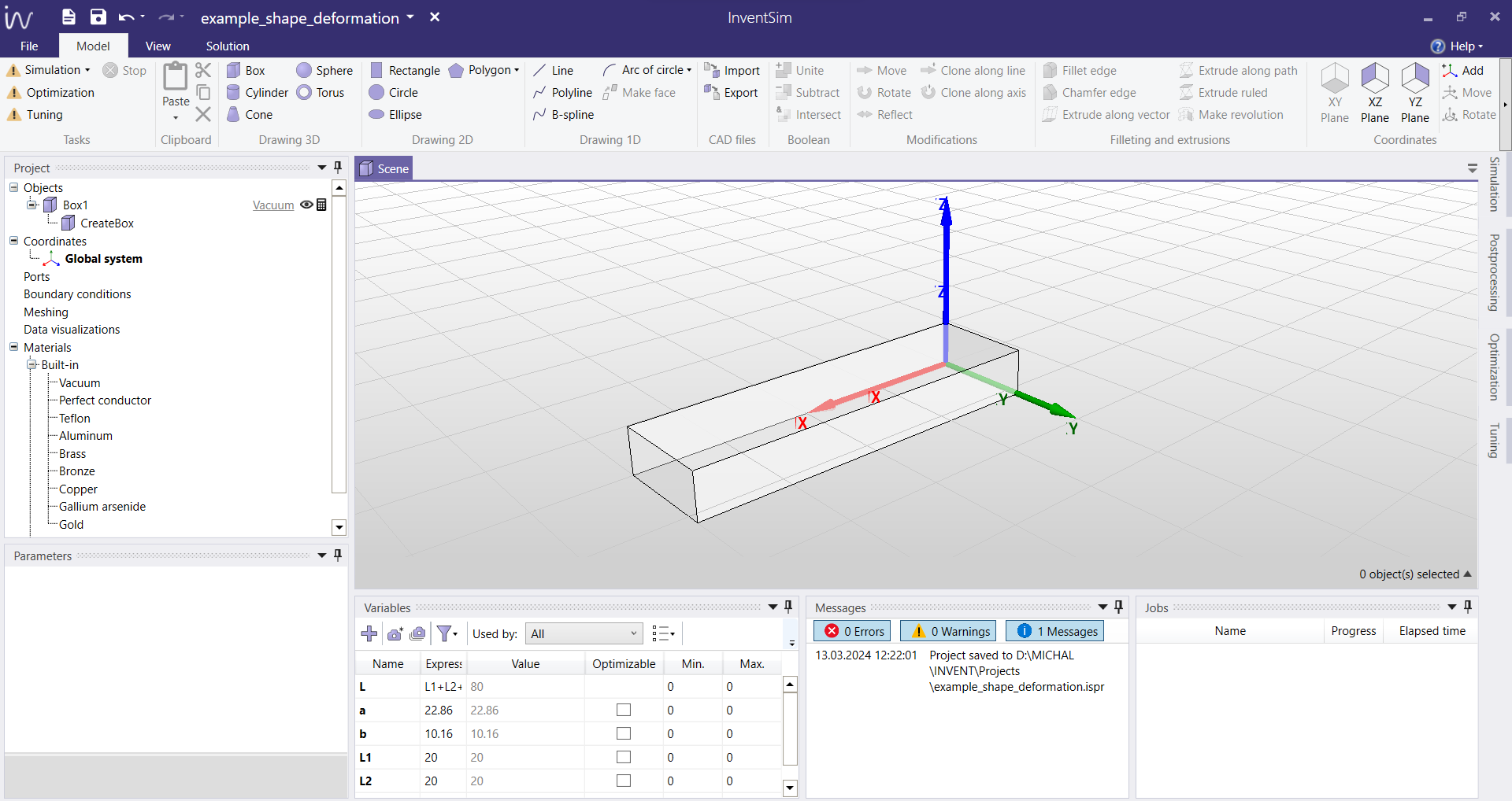
In order to alter the geometry of this structure by shape deformation, a number of control points need to be selected around it. In this example, the control points are defined on a box enclosing the waveguide section. You can do it by creating a new shape deformation definition, by choosing the option "Set mesh operation > Deformation" upon right-clicking on the chosen object, as shown in Fig. 7.7. You can define more than one shape deformation in a single project, but they will be considered as separate operations. If you want to add multiple definitions to a single deformation (i.e., multiple lists of control points to be considered during the same operation), you can choose the option "Set mesh operation > Definition to existing deformation", and add another list of control points to your existing mesh deformation.
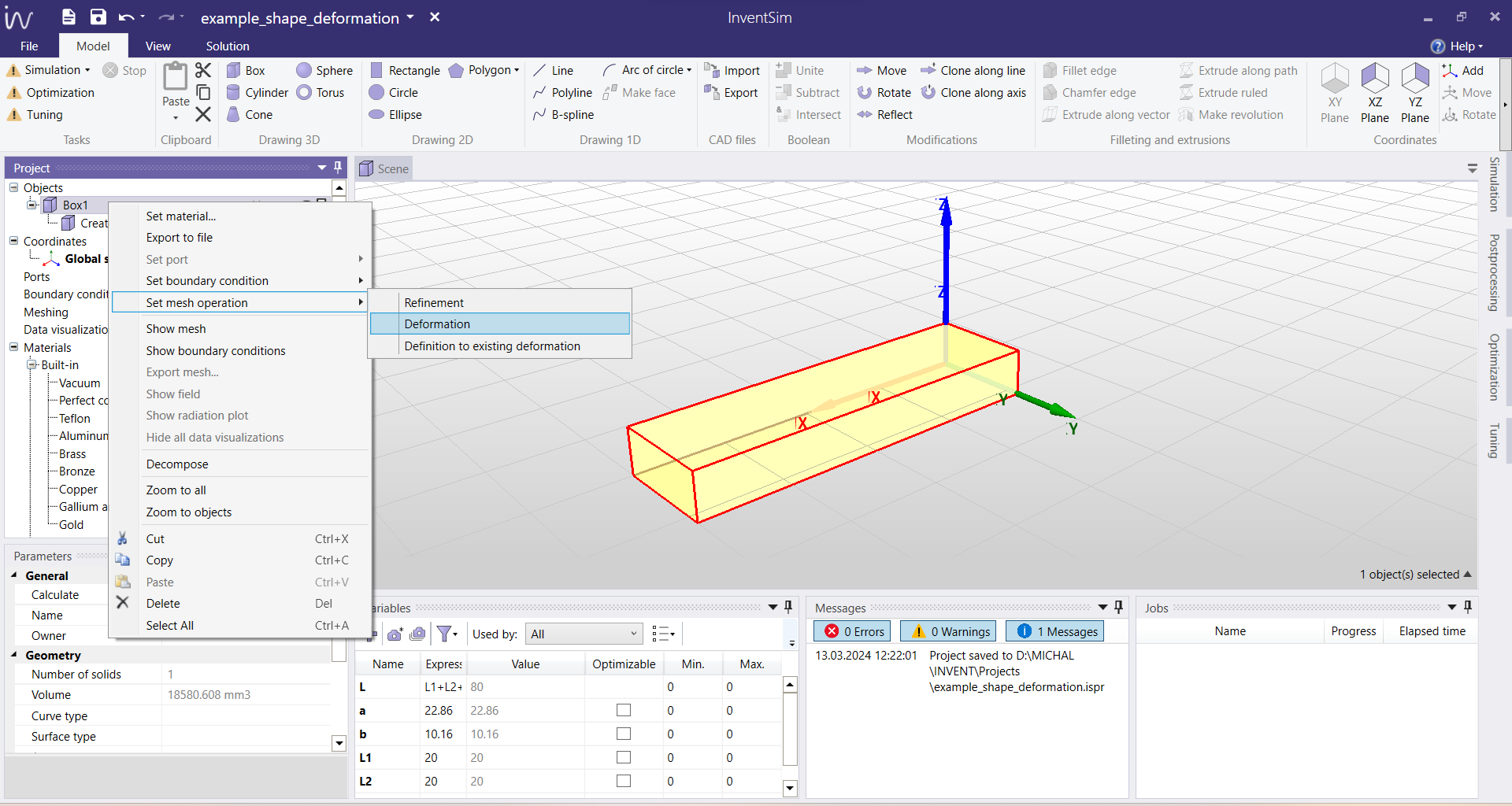
After choosing the option to create a new mesh deformation, an exemplary set of control points is generated automatically around the chosen object, as shown in Fig. 7.8. You can manually change the auto-generated list by selecting the number of divisions, e.g. in each of the three directions defined in Cartesian coordinates: X, Y, and Z. You can modify these points or add more control points afterwards. To be able to modify the auto-generated points, they need to be selected at this point, as highlighted in Fig. 7.9. You can either select each point by clicking on it manually, or select them all by using the key combination "Ctrl" + "A".
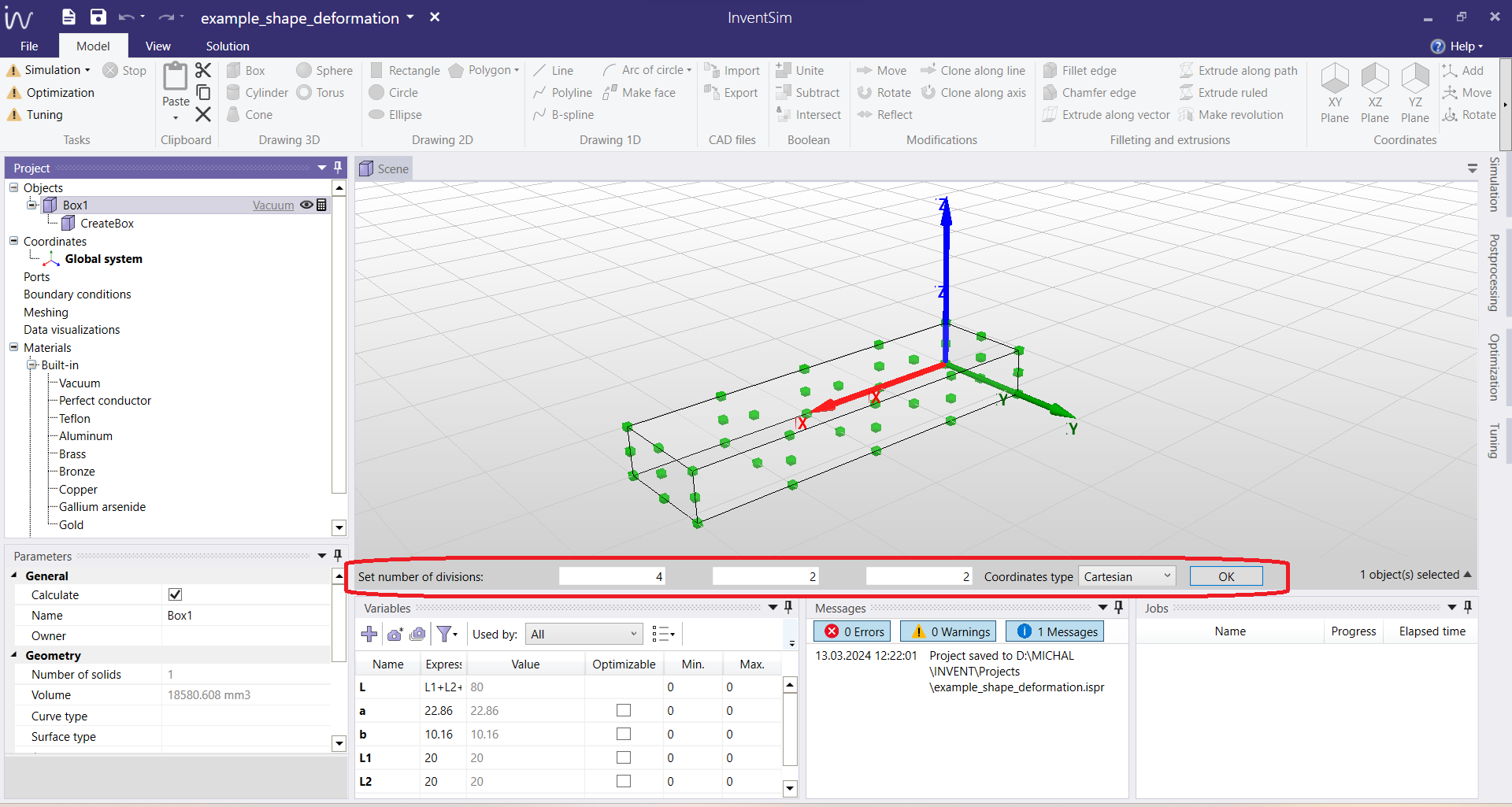
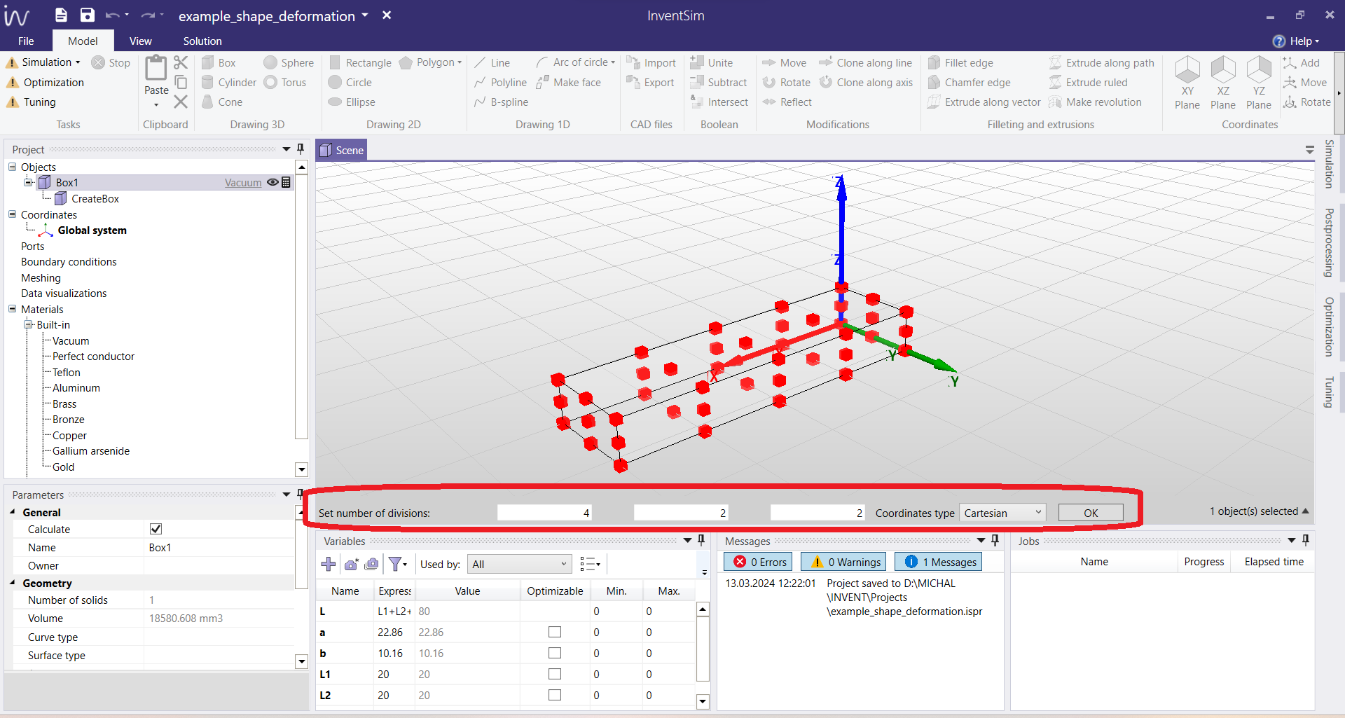
Upon successful creation of the mesh deformation definition, you can find it in the Project tree under Meshing > MeshDeformation1. When selected, you can access its parameters, as shown in Fig. 7.10. From there you can choose the radial basis function to be used in the interpolation, and define its parameters, such as function power and function radius, as was described above in Section 7.5.1. If more than one control points definitions were created, they can all be found under their respective mesh deformation in the Project tree. In this example, there is only one, Definition1, which is linked to MeshDeformation1.
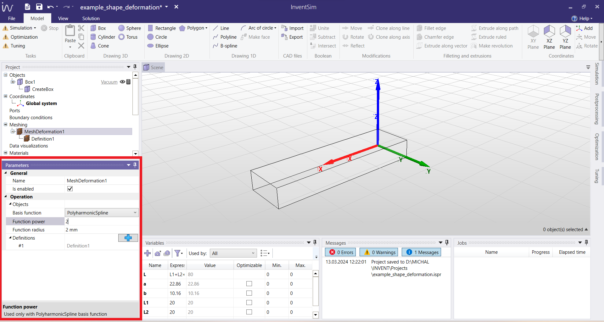
The list of control points and their displacements can be accessed and controlled by choosing the respective Definition (in this example, Definition1). After choosing this option in the Project tree, the user can access the list of control points, as shown in Fig. 7.11. You can edit the coordinates (position) of each point, as well as assign a displacement (offset) to define their movement to a new position. When a non-zero offset is defined, the displacement vector, depicted by a green arrow, becomes visible in the graphical user interface, as in Fig. 7.11. The original structure is deformed depending on the number of control points and the direction of their offsets.
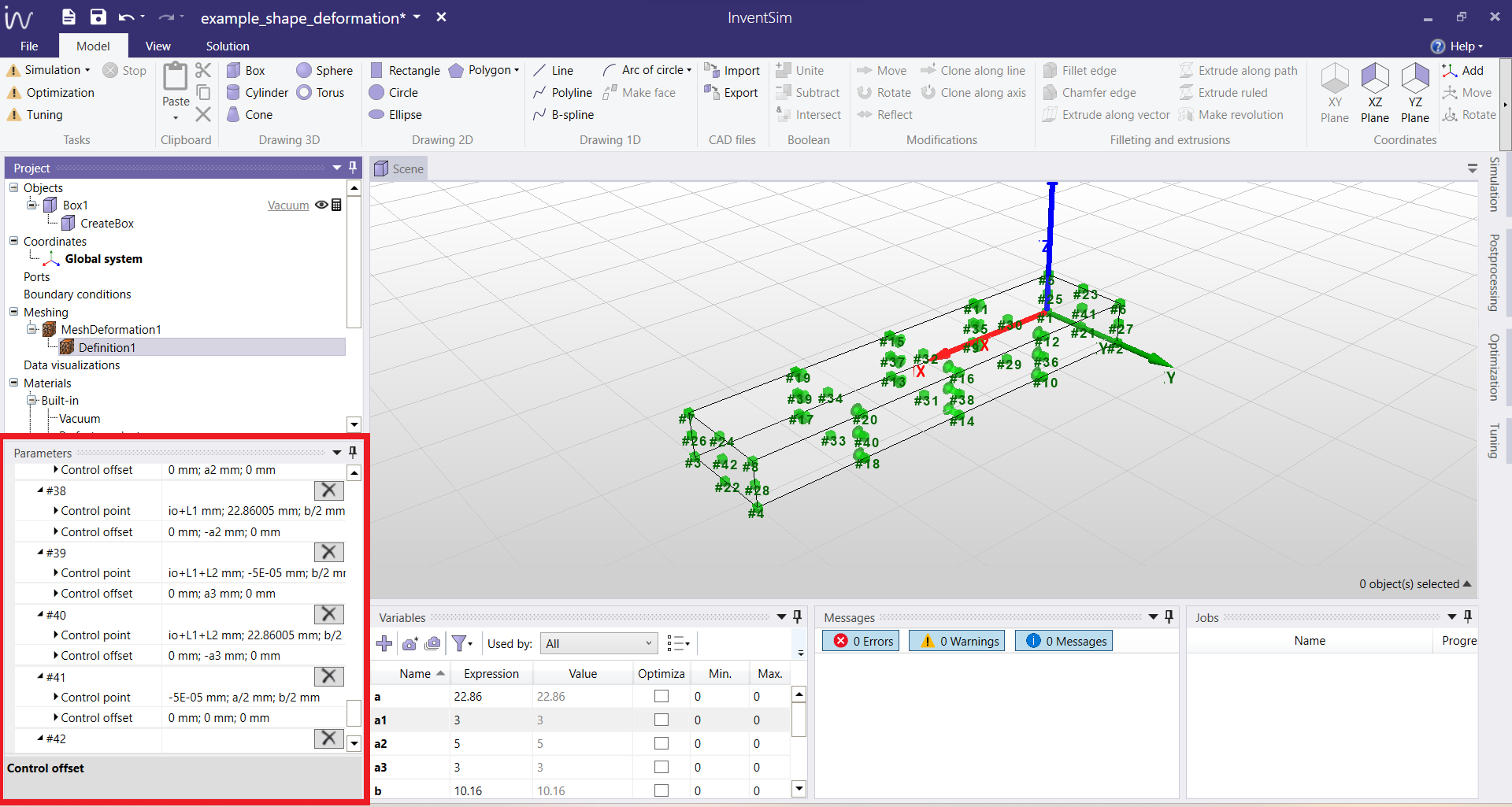
It should be noted that the shape deformation scheme does not limit the number of control points. More complex deformation schemes can easily be employed by adding more control points with movement in arbitrary directions. You can easily add a new control point to an existing deformation by clicking the "+" button located at the heading of the respective Definition containing the list of control points, as presented in Fig. 7.12.
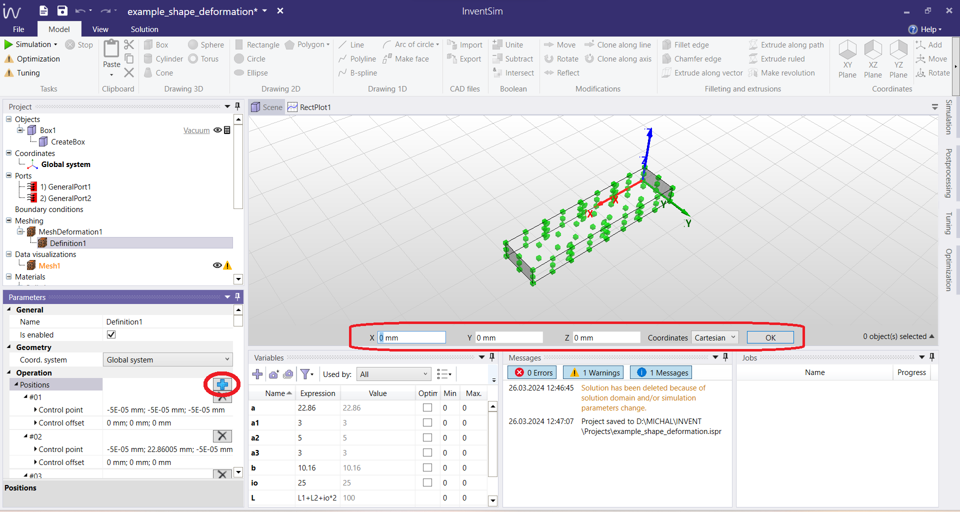
Finally, when the shape deformation parameters and the control points are properly defined, the deformation will be performed during each EM simulation: the deformation is applied to the 3D mesh, just after the mesh generation process. To observe the effect, an EM simulation needs to be run for the project. The parameters used to define the positions and offsets of the control points can be project variables, and they can be used for Tuning and/or Optimization. In this example, a simple squeezing operation was defined for the basic rectangular waveguide section, and the project was optimized to receive a bandpass response, as shown in Fig. 7.13. After the simulation is complete, you can see the deformed 3D mesh by making it visible (right-clicking on the object and choosing the option "Show mesh").
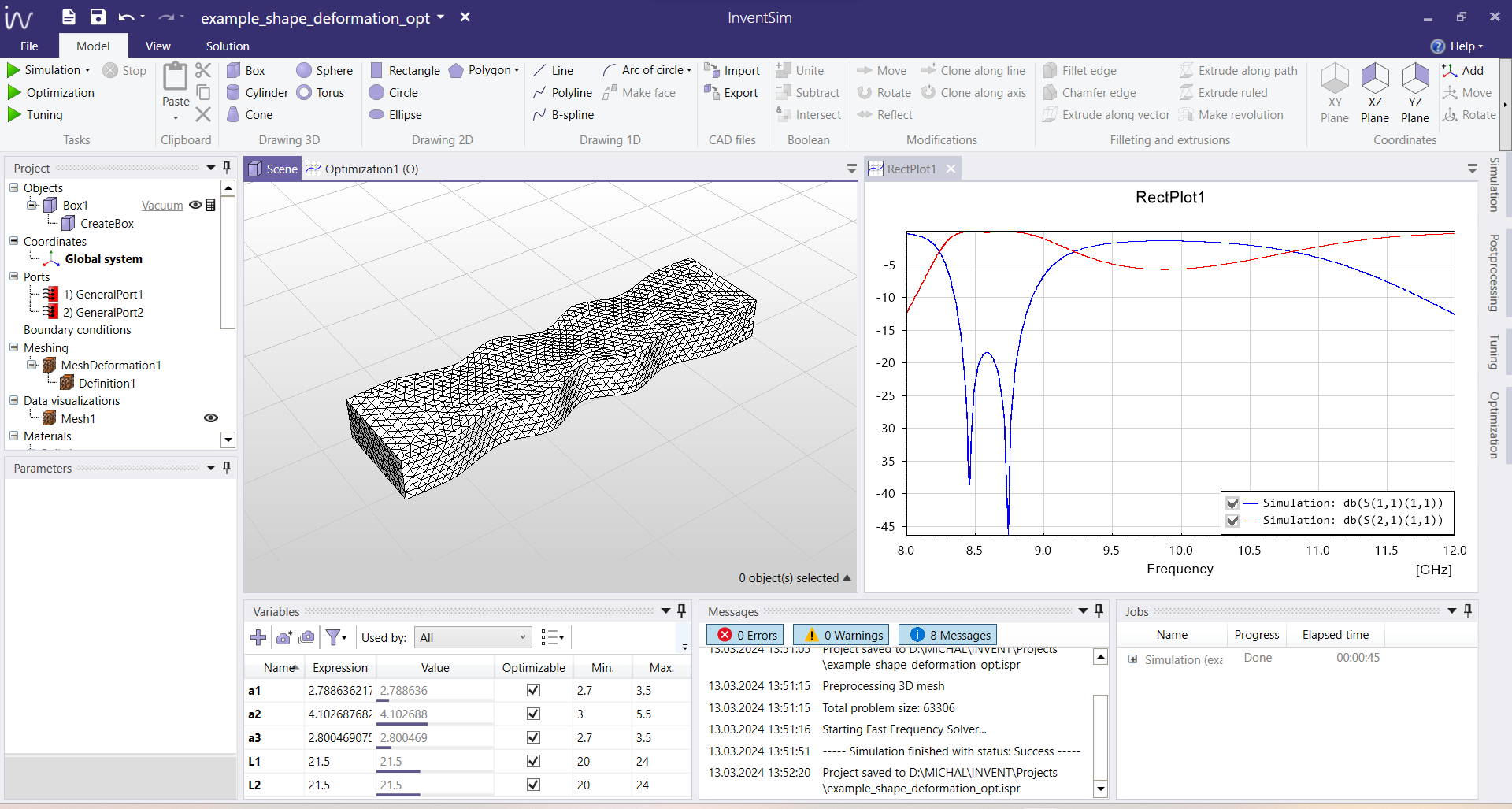
8 Simulation options
Once the model is ready for simulation - i.e. the geometry, materials, boundary conditions, ports and mesh options are properly defined in the project, the last step before starting the simulation is to adjust the solution settings.
In InventSim, several settings for the solution phase are available in the "Solution" tab of the "Simulation" window hidden on the right part of the interface (Fig. 8.1). The settings include:
-
• Setup of simulation frequencies.
-
• Solver options.
-
• Saving solution datasets.
8.1 Frequency plan
The purpose of the frequency sweep simulation is to obtain a structure response in the frequency domain by computing the response at defined frequency points.
Frequency points are defined in the "Frequencies" part of the "Solution" panel. Frequency points are specified in a form of frequency ranges, listed on left of the tab. A frequency range is defined as a set of points that is evenly distributed on the frequency axis, with the following parameters:
-
• Name. The name of the frequency range.
-
• Minimum frequency. The lower bound of the frequency range.
-
• Maximum frequency. The upper bound of the frequency range.
-
• Number of steps. The number of points in the frequency range.
-
• Step size. The distance between the two closest frequency points in the frequency range.
To add a frequency range, select "Add" from the context menu of the left side of the tab. The new frequency range will be added with the default parameters and the default name.
To delete the frequency range, first select it in the list and then choose "Delete" from the context menu.
Frequency ranges can be made inactive in order to temporarily disable the simulation at some frequency points. Only the active frequency ranges are used during the frequency sweep simulation. To activate or deactivate a frequency range, select the checkbox on the left side of the frequency range name.
8.2 Solver options
The solver options are located just below the "Frequency plan" settings. The aim of those options is to give you better control of the solution phase. In general, every 3D FEM simulation of electromagnetic fields in the frequency domain involves a solution of a large, sparse linear system of equations in form:
\(\seteqnumber{0}{}{38}\)\begin{equation} A \cdot x = b \end{equation}
where \(A\) is a sparse matrix, \(b\) is a block of right hand side vectors that correspond to excitations (modes) at ports, and \(x\) is a solution vector that represents the unknown fields inside of the structure. The equation is solved at every frequency point. The size of the linear system matrix \(A\), i.e. the number of the unknowns, depends on the model discretization and the order of the base function used to represent the fields.
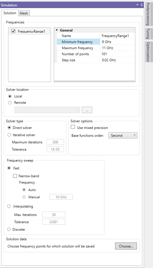
8.2.1 Solver location
You can define the machine on which the solver process will run with this option. The default setting value is "Local" - i.e. the same machine on which the InventSim GUI application is running. The solver can be run, remotely, on another networked machine (with the necessary license) by selecting "Remote" and specifying the IP address and the port of the machine. After entering the machine parameters, use the "Check" button to check the remote solver response.
8.2.2 Solver type
This is the area in which InventSim allows you to setup the numerical techniques that will be used to solve a problem. These are the available options:
-
• Direct solver. With the direct solver, the linear system of equations is solved by using sparse matrix factorization algorithms. In InventSim, we use Intel MKL Pardiso that has this option. In general, a direct solution of the problem is a memory consuming process, but as long as you have have enough memory to be able to factorize the matrix, this is the recommended setting. It is recommended to use this option if possible, especially when "Fast frequency sweep" is enabled.
-
• Iterative solver. With this option, the solution phase is done with the iterative method (PCG) with the dedicated preconditioner. This setting is recommended for very large problems that cannot be solved with the "Direct" solver due to the "out of memory" problem. To use the iterative solver, you need to specify the maximum number of iterations that will be performed for each solution as well as the solution tolerance (defined as residual error of the solution). Please note that the convergence of a iterative solver cannot be guaranteed.
-
• Mixed precision.In order to reduce the memory footprint during the solution phase, some stages of the solution can be performed using a single precision floating point number. Enabling this option will save some memory, but in rare cases it can lead to lower accuracy of the solution.
-
• Base functions. With this option, you can specify the order of the base functions that will be used to represent the electromagnetic field.
-
– First order - the solver uses a linear vector functions defined over tetrahedron element (CTLN - constant tangential, linear normal).
-
– Second order - the solver uses a quadratic vector functions defined over tetrahedron element (LTQN - linear tangential, cubic normal).
-
– Third order - the solver uses a cubic vector functions defined over tetrahedron element (QTCuN - quadratic tangential, cubic normal).
With the increase of the base function order, the problem size increases substantially. In practice we recommend using the default "Second order" option as it is a compromise between the accuracy of the solution and the solution time.
-
8.3 Frequency sweep type
With this option, you can choose between three different frequency sweep techniques: the ’Discrete Sweep’ the ’Fast Frequency Sweep’, and the ’Interpolating Sweep.’ The last two can expedite the evaluation of the transfer function at multiple frequency points.
The most general sweep is ’Discrete sweep.’ When selected, simulation is performed independently for every frequency point, which means that at each frequency point, a large linear problem has to be solved. If a substantial number of frequency points is defined in the frequency plan (tens or hundreds), this can lead to a long simulation time. At the same time, this option provides the most rigorous results. It is also recommended to use the discrete sweep when the number of points defined in the simulation is very low (i.e. below 10).
With the "Fast frequency sweep" enabled, the model of the transfer functions is constructed in an adaptive way: as the order of the model grows, the convergence of the transfer function is monitored. Usually, the numerical cost of creating such a model is much lower than a discrete sweep. In this mode, the wideband response in the frequency domain is extracted from the solution at a minimum number of frequency points - in some cases we can extract the wideband response even from a single frequency point! The efficiency of the fast frequency sweep depends on the number of resonances within the structure over the analyzed frequency band. If there are many resonances (tens/hundreds), the sweep may become less efficient, or could even fail. In this case, the direct sweep is recommended. Please note that the ’Fast Frequency Sweep’ cannot be used for simulation projects that involve dispersive materials like Debye dielectrics, ferrites, or RLC boundary conditions.
Optionally, one can use the ’Narrowband’ option within the ’Fast Frequency Sweep.’ This option is suitable when a narrow or medium frequency bands are concerned, and the algorithm enforces the extraction of the transfer function from single frequency point simulation. If this option is selected, the user can provide the solution frequency from which the algorithm will start - only at this frequency can the field be saved and post-processed.
The last option is ’Interpolating Sweep’ which relies on the adaptive construction of a rational model for the system’s response. In this case, the algorithm dynamically selects frequency points and strives to create an accurate model of the transfer function within the specified frequency range. This sweep is compatible with frequency-dependent materials and boundary conditions. The user can define the number of iterations, which corresponds to the maximum number of solutions allowed to create the model, as is strictly connected to the predicted maximum order of the transfer function.
8.4 Solution/Field data saving
When using the default simulation settings, InventSim does not save the information about computed fields. InventSim simply calculates the transfer function between the ports defined in the project. In order to save the fields at user-defined frequencies, move to the simulation settings and the "Solution data" section on the bottom (Fig8.2). Select the "Choose" button and a new window will appear (Fig.8.3) with the list of all simulation frequencies. Select those that are of interest to you.
Remarks:
-
• Only if the field information is saved can you evaluate and display the fields or post-process the near fields using the near-to-far field transformation.
-
• If the fast-frequency sweep is used in the "Narrowband" mode, the field information is available only at a solution frequency that is set in the fast frequency sweep options.
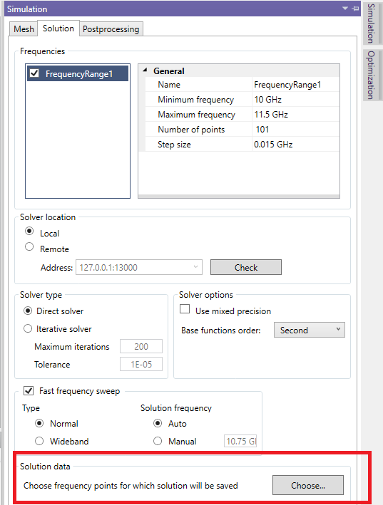
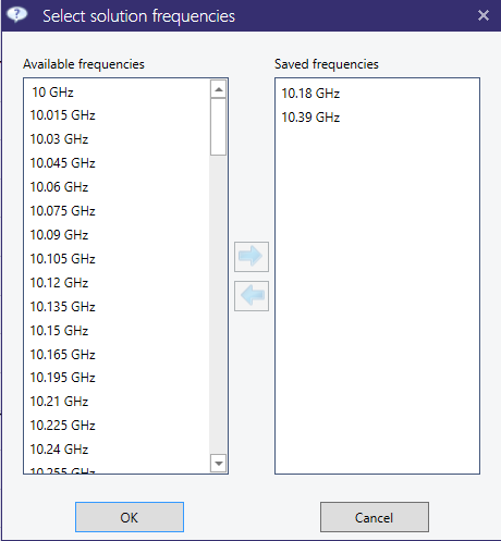
9 Postprocessing
Once the simulation is completed, it is possible to perform postprocessing of the calculated field solutions, which includes:
-
• Displaying the calculated transfer function,
-
• Visualization of computed electric and/or magnetic fields,
-
• If the absorbing (radiation) boundary condition is present, transform the near field to the far field and display the radiation pattern as a 2D or 3D plot and evaluate the radiation parameters (gain, efficiency, etc.).

The postprocessing tasks are available in the "Postprocessing" panel on the right side of main InventSim window - Fig. 9.1. With this option you can add, modify and remove postprocessing tasks defined in current project.
Evaluation of the transfer function is a default task in InventSim - no additional postprocessing task is needed to display the transfer function.
9.1 2D Plots of transfer functions
A core functionality of InventSim is calculating the transfer function between ports defined in the project. By default, InventSim computes and displays the transfer function in the form of plots of scattering parameters. If the project does not have a defined plot and the simulation is about to finish, you will need manually add a default plot for computed scattering parameters.
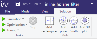
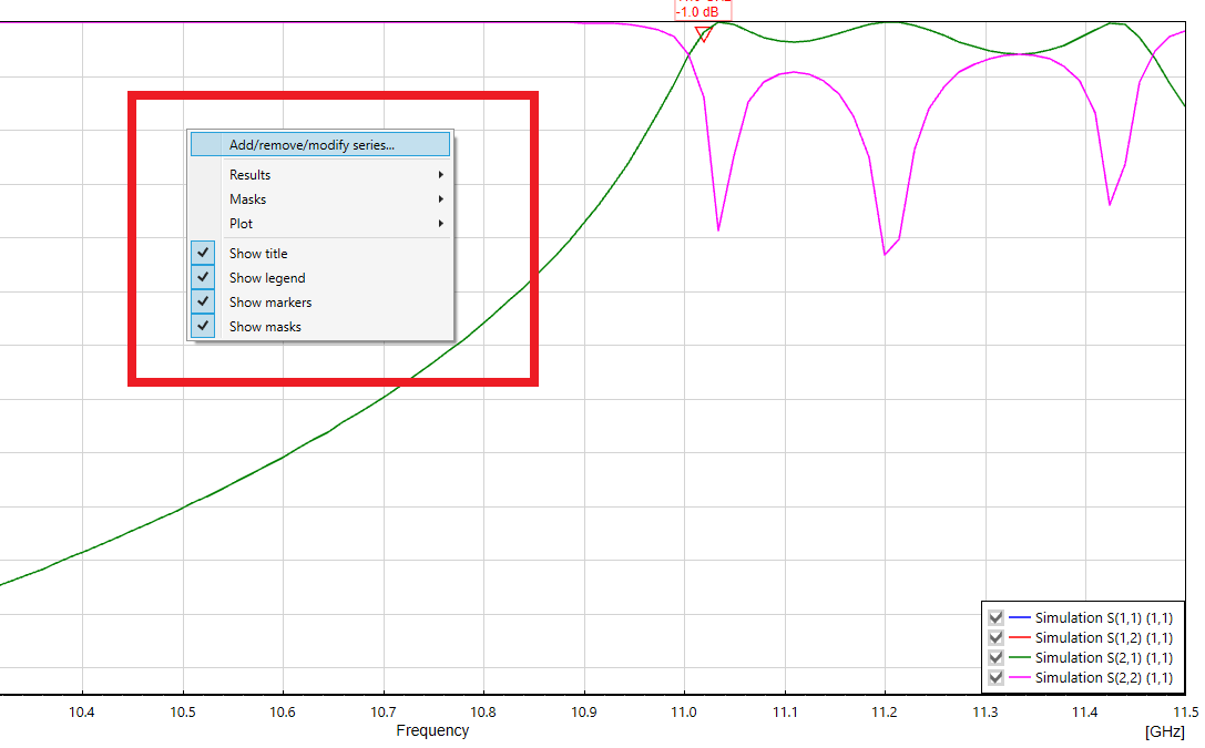

The plot type options is accessible in the "Solution" window located in the upper part of the main application window (the toolbar shown in the picture 9.2). Few plot types are available:
-
• Rectangular. Basic 2D plot with (X,Y) axes.
-
• Smith. Smith chart used to display impedance/admittance parameters.
-
• Polar. Basic 2D polar plot for visualization of radiation patterns.
-
• 3D. 3D plot in spherical coordinate system for visualization of radiation patterns in 3D.
The results of port-driven simulation can be plotted as S,Y,Z, VSWR or group delay parameter plots. For of each set of data series, the user can also apply the additional modifiers, like:
-
• Magnitude
-
• Magnitude in dB
-
• Phase
-
• Real part
-
• Imaginary part
-
• ...
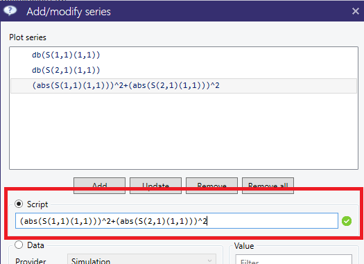
It is also possible to use the data set and invoke the user-defined script, based on mathematical formula provided by the user - overriding the software preset. For example, the power budget \(P\) of two-port network can be calculated based on formula \(P = \mid S_{11} \mid ^2 + \mid S_{21} \mid ^2 \). The example of such definition is shown in Fig.9.5. The list of functions that can be used to define a custom data series via the script functionality is shown table 4.
The plot type can be changed from the context menu by selecting "Add/remove/modify series...".
Each of the plotted parameters is represented by a data series and it is plotted as a line. The plot series are listed in the legend on the right side of the plot. The default name for simulation results is "Simulation" with the ID of the port. You can temporarily remove the plot series from the plot by deselecting the checkbox located on the left side of the legend item.
Zooming on the plot is achieved by selecting the region of the plot with the mouse while pressing the left mouse button. To zoom out from the plot, choose "Reset zoom" from the context menu of the plot. Alternatively, exact axes limits can be set in the "Options" panel at the bottom of the plot.
| Symbol | Description |
| ̂ | Power |
| + | Add |
| - | Subtract |
| / | Divide |
| * | Multiply |
| sin() | Sinus |
| cos() | Cosinus |
| tan() | Tangent |
| cosh() | Hyperbolic cosinus |
| sinh() | Hyperbolic sinus |
| tanh() | Hyperbolic tangent |
| conj() | Complex conjugate |
| real() | Real part |
| imag() | Imaginary part |
| phase() | Phase of complex data series |
| mag() | Magnitude |
| ‘ complex() | ? |
| abs() | Module |
| max() | Maximum value of data series |
| min() | Minimum value of data series |
| pow(,n) | Power function |
| log10() | Common (base-10) logarithm |
| log() | Natural logarithm |
| db() | 20log10(\(\cdot \)) |
| db10() | 10log10(\(\cdot \)) |
| ceil() | Smallest following integer |
| floor() | Largest previous integer |
| sqrt() | Square root |
| exp() | Exponential |
| normalize() | Normalize data series to max. value |
9.1.1 Markers
To attach a marker to the current plot, select the data series to which the marker will be added (the series line will be highlighted) and use the context menu (Fig.9.6). Once the marker is added at a specific point of the plot, it can be moved to a different point by using the mouse.
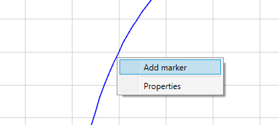
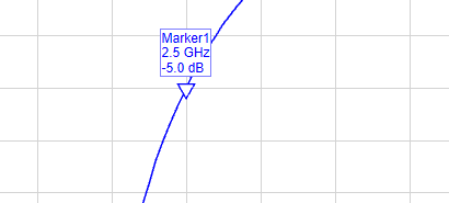
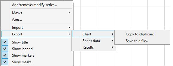
9.1.2 Exporting data.
The simulation data can be exported to a file by using the context menu on the plot and selecting submenu "Export ->". The data can be exported on different ways (Fig.9.7):
-
• As a graphic of the active chart window. The available output formats are: .PNG, .GIF, .JPG, .BMP and .TIFF. Using the same context menu, you can also copy the current plot to the clipboard.
-
• As data series to CSV file,
-
• As simulation result file using Touchstone file format.
9.1.3 Zoom/Move/Autoscale 2D plot
To zoom in on the plot area, click LMB on the plot and select the upper corner of the area that needs to be seen in greater detail. Then, move the mouse to the right and down to mark the requested area. To move the plot, use the right mouse button and simply drag the plot.
To restore the view of the plot after the zoom option has been used, click the LMB on the plot area and move the mouse to the right as well as up.
9.2 Smith chart
The admittance/impedance parameters can be plotted on the "Smith" chart. The "Smith" chart can be added using the "Plots" section in the "Solution" toolbar. (Fig. 9.2). Please note that since the electric field formulation is used, we compute the admittance parameters directly, but the reference impedance to transform the Y-parameters to S-parameters is a modal (wave) impedance, applying a relation [9]:
\(\seteqnumber{0}{}{39}\)\begin{equation} S = 2 \cdot (I+Y)^{-1} - I \end{equation}
where \(I\) is a unitary matrix. Please also note that in the case of wave ports (non TEM-mode), the characteristic impedance is not unique. Only in the case of lumped ports can we re-normalize the scattering parameters to characteristic impedance and then to 50\(\Omega \) standard. Example of a Smith chart is shown in Fig.9.8.
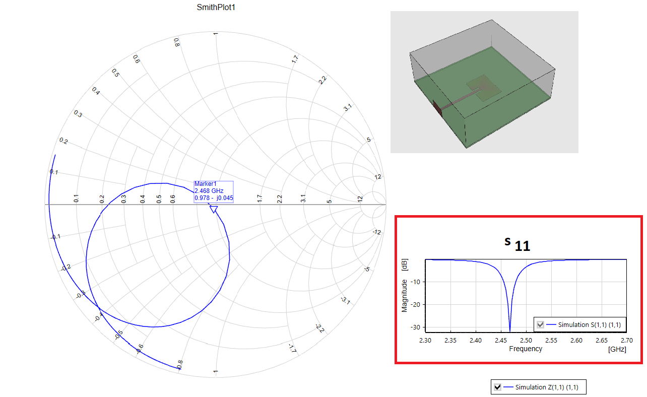
9.3 Field visualization
InventSim provides near field visualization capabilities which allows to render either scalar (i.e. magnitude of the field) or vector form of the electromagnetic field in Scene panel. The scalar form can be displayed as 3D isosurfaces (surfaces of constant field magnitude) or 2D isolines on a cut plane. The vector form is displayed as arrows which direction represent the direction of the field and length/color representing the E/H field magnitude.
9.3.1 Adding
Visualizations require data calculated in postprocessing stage based on field solution saved for the user-defined frequency points, as described in section 8.4. The necessary postprocessing task can be added by selecting "Add field solution" from the context menu of "Postprocessing" tab in "Simulation" panel. The task is then added with a default frequency set. The frequencies can be changed by clicking "Modify" button and selecting the desired frequency in the dialog window. Please note that the selected post-processing frequency must be defined within the frequency sweep. If the user changes the simulation frequency plan in a way that removes the post-processing frequency point, the simulation will not be executable.
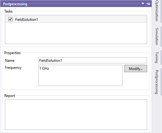
Alternatively, the postprocessing task can be added automatically while adding the visualization. To do so select "Show field" in Scene context menu which will open a wizard window consisting of three wizard pages. The first one allows to choose a data source in a form of a postprocessing task. User can either choose an existing postprocessing task or add a new one with a specified frequency list. As each postprocessing task is executed independently, please make sure to reuse and share existing tasks when creating multiple field plots.
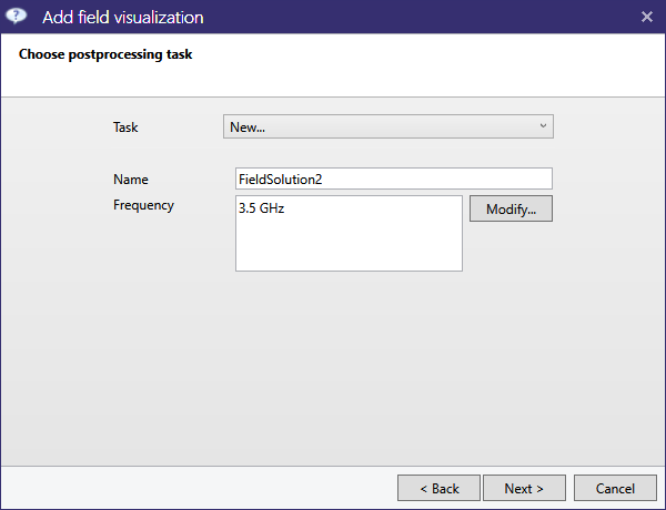
The second page lets choose the visualization type: isosurface/isoline or vector type:
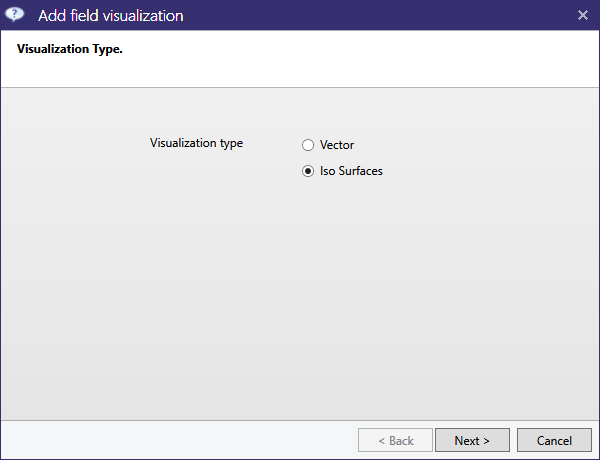
Finally, general visualization parameters are specified i.e. frequency, port and mode of the excitation, field type and coordinate system.
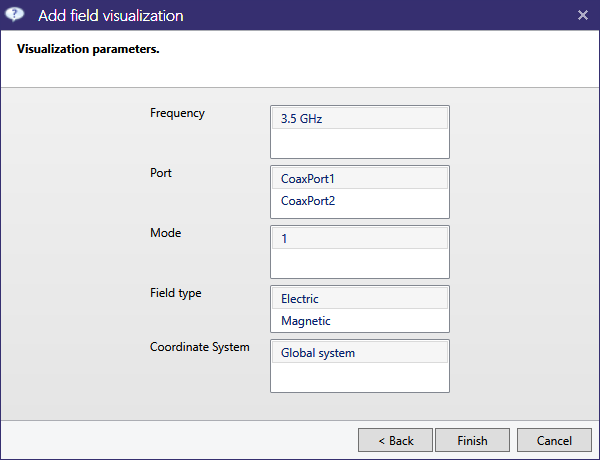
Clicking "Finish" button closes the wizard window and adds postprocessing task as well as field visualization to the project. It also starts postprocessing task calculation and visualization generation task. Once the tasks are finished, field visualization is displayed in Scene. The examples of field visualization are shown in Figures 9.13 and 9.14.
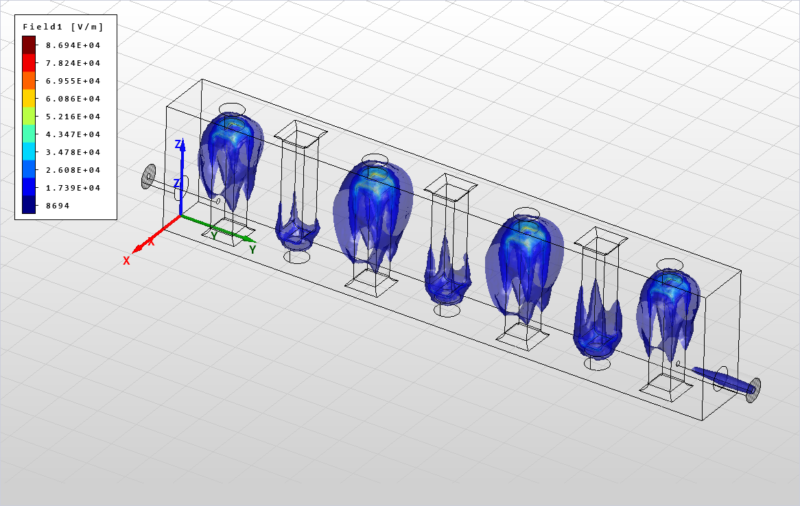
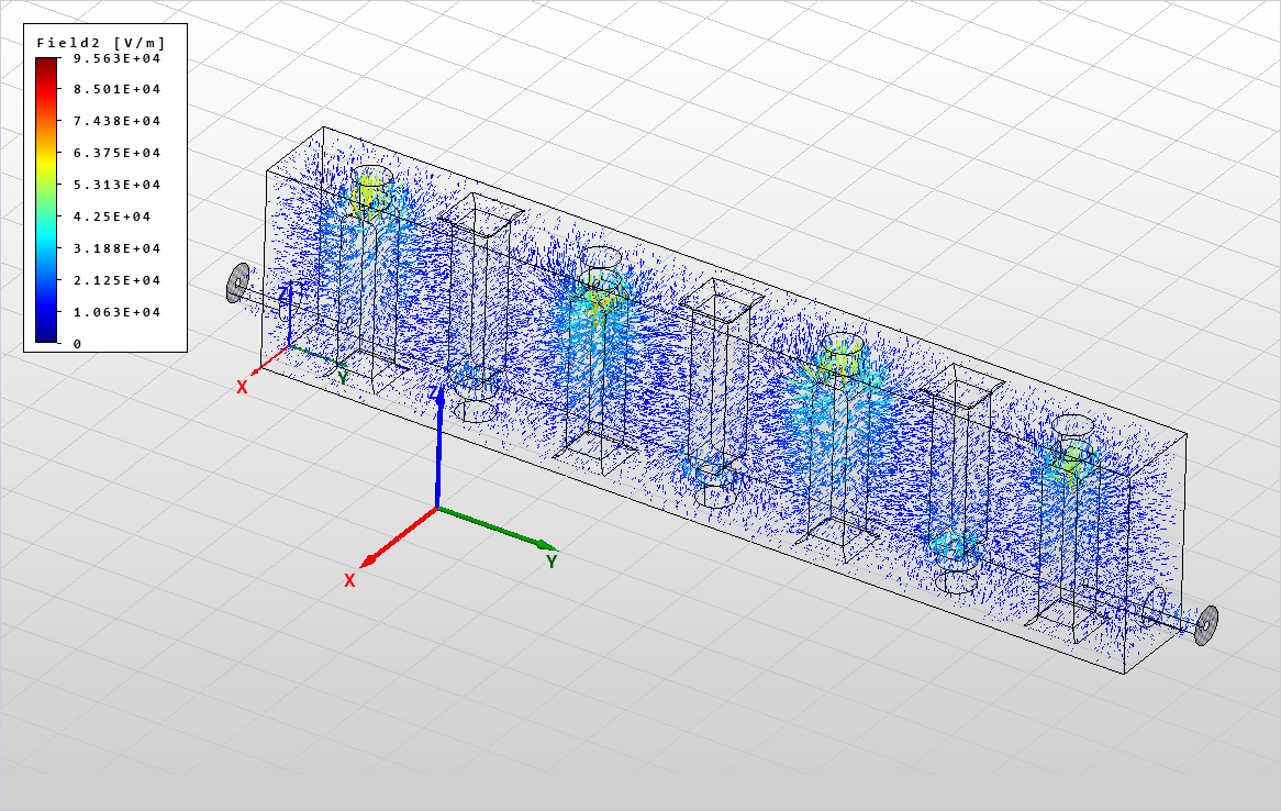
Each field visualization has a corresponding legend displayed on the left part of the screen, as shown in figures above. When isosurfaces/isolines are displayed, the legend shows a set of colors, each representing a field value displayed as a isosurface/isoline. Please note that there is no isosurface/isoline representing neither minimum nor maximum value of the field. In case of vector field visualization the legend shows continuous set of colors as displayed arrows representing field value and direction can have any value, including minimum and maximum values as well.
9.3.2 Parameters
Field visualization have a number of parameters to customize the displayed result. The common set of parameters is:
| General | |
| Name |
Name of the visualization |
| Is visible |
Shows or hides the visualization |
| Object |
Object for which field visualization is generated (not used) |
| Visualization | |
| Postprocessing task |
Name of postprocessing task, the data source of the visualization |
| Color map |
Color map used to color isosurfaces, isolines and vectors |
| Field type |
Electric or magnetic field |
| Coordinate system |
Coordinate system used in iso lines cut plane definition |
| Auto limits |
If true visualization is always displayed based on the current min and max values |
| Max value |
If Auto limits is set to false, this value is used to display visualization |
| Min value |
If Auto limits is set to false, this value is used to display visualization |
| Excitation | |
| Frequency |
Excitation frequency |
| Port |
Excitation port |
| Mode |
Excitation mode |
| Phase |
Excitation phase |
Additionally scalar field visualization have parameters:
| Isosurfaces | |
| Is visible |
Indicates whether to display isosurfaces |
| Count |
The number of isosurfaces |
| Isolines | |
| Is visible |
Indicates whether to display isolines |
| Count |
The number of isolines displayed |
| Colored surface |
If set to true, cut surface will be colored |
| Offset value |
Offset value in the current cut axis in Coordinate system |
| Cut axis |
The axis defining the cut plane |
Vector field visualization have additional parameters:
| Vector field | |
| Scale |
Set scaling factor for displaying the arrows |
| X Count |
The number of sections in X axis |
| Y Count |
The number of sections in Y axis |
| Z Count |
The number of sections in Z axis |
| Is irregular |
If set true, vector positions will be generated randomly |
| Is visible |
Indicates whether the arrows are displayed |
9.4 Radiation patterns
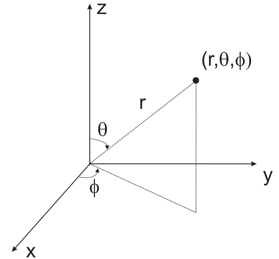
To simulate open structures in InventSim, you should apply the absorbing boundary condition (ABC). This allows the truncation of the computational domain and solving the problem that has a reduced size. Once the simulation is completed and the structure fields are saved for the frequencies defined by the user (look how to define those frequencies in section 8.4), InventSim allows you to calculate the radiating fields in the far field zone using a near-to-far field transformation. In this case, the outer surfaces for which the boundary condition is defined are the source of the external far field. The far field zone distance/radius has to be defined by the user.

You need to add a postprocessing task to calculate the radiation patterns. It can be done in two ways:
-
• Selecting the "Postprocessing" tab in the "Simulation" options window and using the context menu to add a new task,
-
• Using the context menu of the 3D geometry modeler and selecting the "Show radiation" item.
Definition of the near-to far field task requires you to provide the observation angles in a spherical coordinate system (Fig. 9.15).
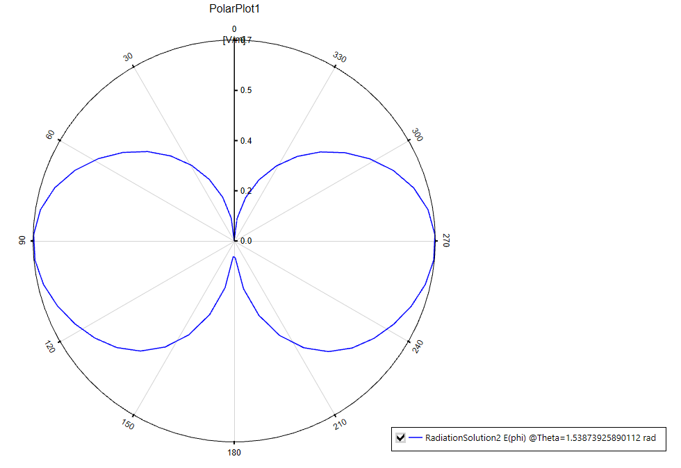
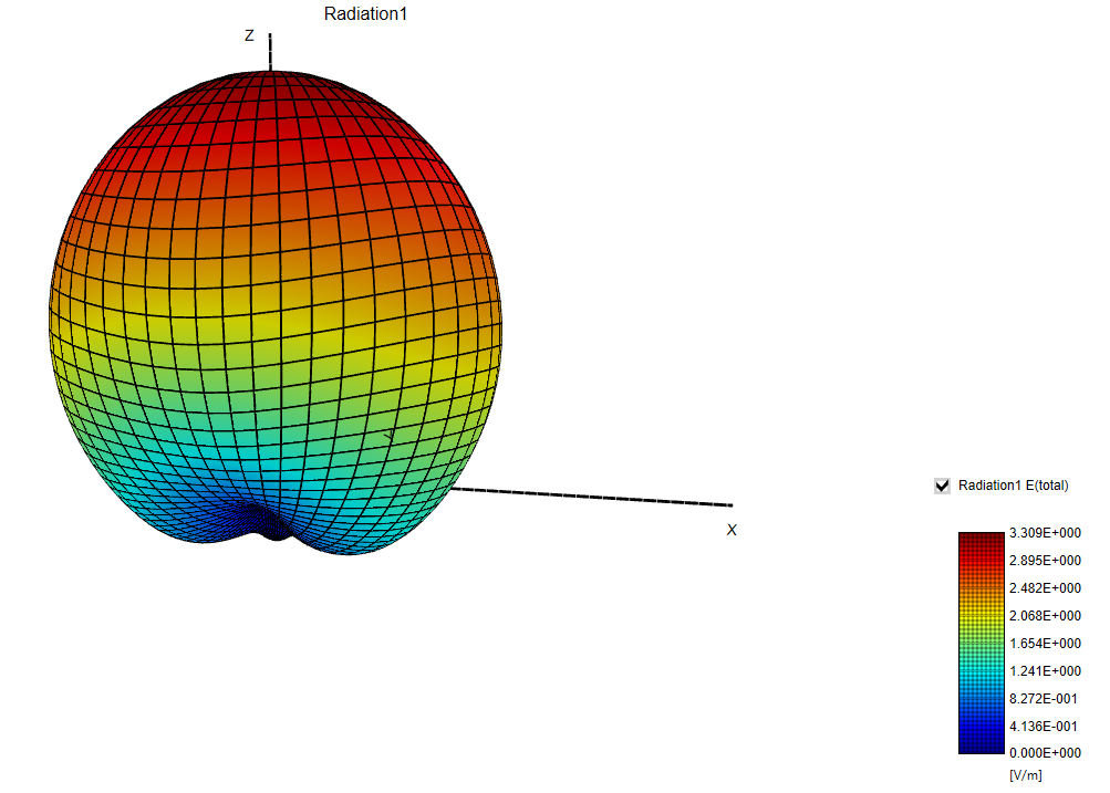
A set of the observation angles is defined for both \(\theta \) and \(\phi \) coordinates with a minimum and a maximum angle value and a number of \(N\) observation points that are uniformly distributed within this range (Fig.9.16). You can define a task of computation of the fields for a single cut (for constant \(\theta \) or \(\phi \) angles, with \(N\)=1) and create a plot in rectangular or polar coordinates (Fig.9.17) You can also compute the fields with both varying angles \(\theta \) and \(\phi \). The latter allows you to compute a 3D plot of radiation patterns, as shown in Fig 9.18.
9.4.1 Near-to-far field transformation
The near-to-far field transformation is implemented using the approach that is described in [27]. In the far field region (in the radial distance \(R > \frac {2D^2}{\lambda }\), where \(D\) is the largest dimension of radiation source), the electric field components in spherical coordinate system can be evaluated from near-electric and magnetic fields using these relations:
\(\seteqnumber{0}{}{40}\)\begin{equation} E_{\theta }(r) = - \frac {jk_0 e^{-j k_0 r} }{4 \pi r } (L_{\phi } + Z_0 N_\theta ) \end{equation}
\(\seteqnumber{0}{}{41}\)\begin{equation} E_{\phi }(r) = \frac {jk_0 e^{-j k_0 r} }{4 \pi r } (L_{\theta } - Z_0 N_\phi ) \end{equation}
where \(\vec {L}(r)\) and \(\vec {N}(r)\) are computed as integrals over surface \(S\) that encloses the source of the radiation:
\(\seteqnumber{0}{}{42}\)\begin{equation} \vec {N}(\hat {r}) = \iint _S \vec {M}(r') e^{j k_0 r' \cdot \hat {r} } dS \end{equation}
\(\seteqnumber{0}{}{43}\)\begin{equation} \vec {L}(\hat {r}) = \iint _S \vec {J}(r') e^{j k_0 r' \cdot \hat {r} } dS \end{equation}
and
\(\seteqnumber{0}{}{44}\)\begin{equation} \vec {J} = \vec {n} \times \vec {H} \end{equation}
\(\seteqnumber{0}{}{45}\)\begin{equation} \vec {M} = - \vec {n} \times \vec {E} \end{equation}
In this notation, \(\hat {r}\) is a unitary vector pointing to the observation point, \(r'\) is a vector of source location and \(\vec {n}\) is a vector that is normal to the surface S. According to the electromagnetic field theory, the radial components of the field vanish in the far field zone and only the transverse (\(\theta \), \(\phi \)) field components are present.
The computation of the far field is done internally. You need to specify the observation points (using the spherical coordinate system). Once the fields are computed, they can be displayed either as a 2D or a 3D plot.
Please note that the near-to-far field transformation might be a computationally intensive process.
9.4.2 Radiation parameters
When the radiation task is defined and solved, InventSim automatically calculates selected antenna/radiation parameters and reports them in a post-processing task panel, as shown in Fig.9.19. The report includes:
-
• Total radiation efficiency - ratio of the total power radiated by a component to the net power delivered by the source. The source is normalized to available power equal one Watt (1W).
-
• Radiation efficiency - ratio of the total power radiated by a component to the net power accepted by the antenna from the source.
-
• Power delivered to component.
-
• Power radiated (real part of complex-valued radiated power.)
-
• Power reactive (imaginary part of complex-valued radiated power.)
9.4.3 Antenna gain
Antenna gain is defined as the ratio of the intensity, in a given direction, to the radiation intensity that would be obtained in the power accepted by the antenna were radiated isotropically. The radiation intensity corresponding to the istropically radiated power is equal to the power accepted (input) by the antenna divided by \(4\pi \) (definition by C.A. Balanis, "Antenna Theory: Analysis and Design".):
\(\seteqnumber{0}{}{46}\)\begin{equation} Gain = 4\pi \frac {U(\theta , \phi )}{P_{in}} \end{equation}
where \(U(\theta , \phi )\) is a radiation intensity
\(\seteqnumber{0}{}{47}\)\begin{equation} U(\theta , \phi ) = \frac {R^2}{2\eta } \cdot \| E(\theta , \phi ) \|^2 \end{equation}
with \(R\) given as a far field zone radius, and \(E(\theta , \phi )\) far-field zone electric field of antenna, and \(\eta =120\pi \) is free space impedance. With this notation, the antenna gain can be evaluated in InventSim using an equation
\(\seteqnumber{0}{}{48}\)\begin{equation} Gain = 4\pi R^2 \frac { \| E(\theta , \phi ) \|^2}{2\eta \cdot P_{in}} \end{equation}
Assuming \(P_in = 1W\), and \(R=1m\) (default values in InventSim), one gets:
\(\seteqnumber{0}{}{49}\)\begin{equation} Gain = 4\pi \frac { \| E(\theta , \phi ) \|^2}{2\eta } \end{equation}
The formula can be then directly implemented in InventSim plot with a script functionality, as shown in Fig.9.20.
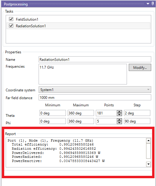
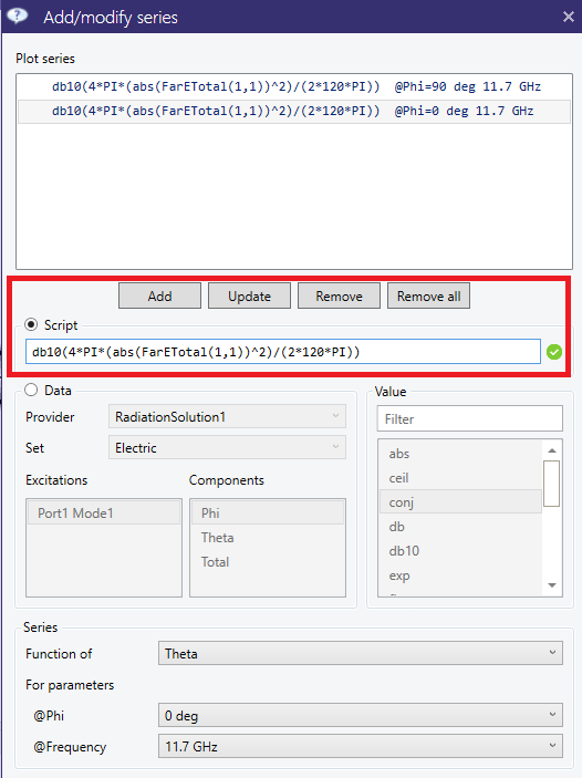
10 Design Tuning and Optimization
In practice, a single electromagnetic simulation of a complex model is rarely used. Usually a series of computer simulations is performed to optimize the computer model. This is done to achieve the required properties of the structure. InventSim was created to simplify this task by either using manual tuning or the automated optimization schemes. In both cases, one of the most important tasks is the proper structure parameterization using variables, as well as the definition of the design parameters/variables. These variables are called "optimization variables" in InventSim.
10.0.1 Optimization variables
Optimization variables are a special type of variables that is introduced to tune or optimize the model. To change the variable type from a regular to an optimization variable, you need to use the IsOptimizable checkbox in the variable properties. Then you can setup the available range of the variable values. This is the range of the variables that will be then accessed and modified by the optimization/tuning module. Optimization variables are marked with a check-box on the list of variables. The colored line below the value text field corresponds with the relative value of the variable in the range of the allowed values. (Fig. 10.1). Please note that only those variables that have numerical expressions can be made optimizable.
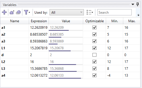
10.0.2 Structure parameterization
Proper structure parameterization is a key part of every design tuning. In general, parameterization should allow you to change the model using the design parameters in a way where each combination of allowed values of the design parameters of the model will remain valid. This, for example, means that no structure will break or unintentionally disconnect from the signal path. In order to achieve the proper parameterization, you can use a combination of variables, equations and relative coordinate systems.
10.1 Design tuning
A unique feature of InventSim is the design tuning module. It allows for fast tuning of the transfer function of the model (e.g. scattering parameters). In order to use the tuning feature, the fast frequency sweep or interpolating sweep must be enabled!
To run the tuning, select the "Tuning" tab and click the "Start" button, Fig.10.2. You can access of the optimization/tuning variables defined in the project in the tuning window. Once the "Start" button is clicked, the solver will simulate the structure. Afterwards, you can modify the values of geometric variables using sliders and see the predicted response of the circuit on the response plot (Fig.10.3). The plot shows both the original response as well as the predicted response which are evaluated for the updated values of variables. The evaluation of this response should not take much time - the plot is updated almost instantly.
Once the response is satisfactory, it can be validated with the "Validate" button click. The solver will then start the evaluation of the true response of the circuit with a new electromagnetic simulation. Once the simulation is finished, you can continue with the next iteration of the design tuning (Fig.10.4).

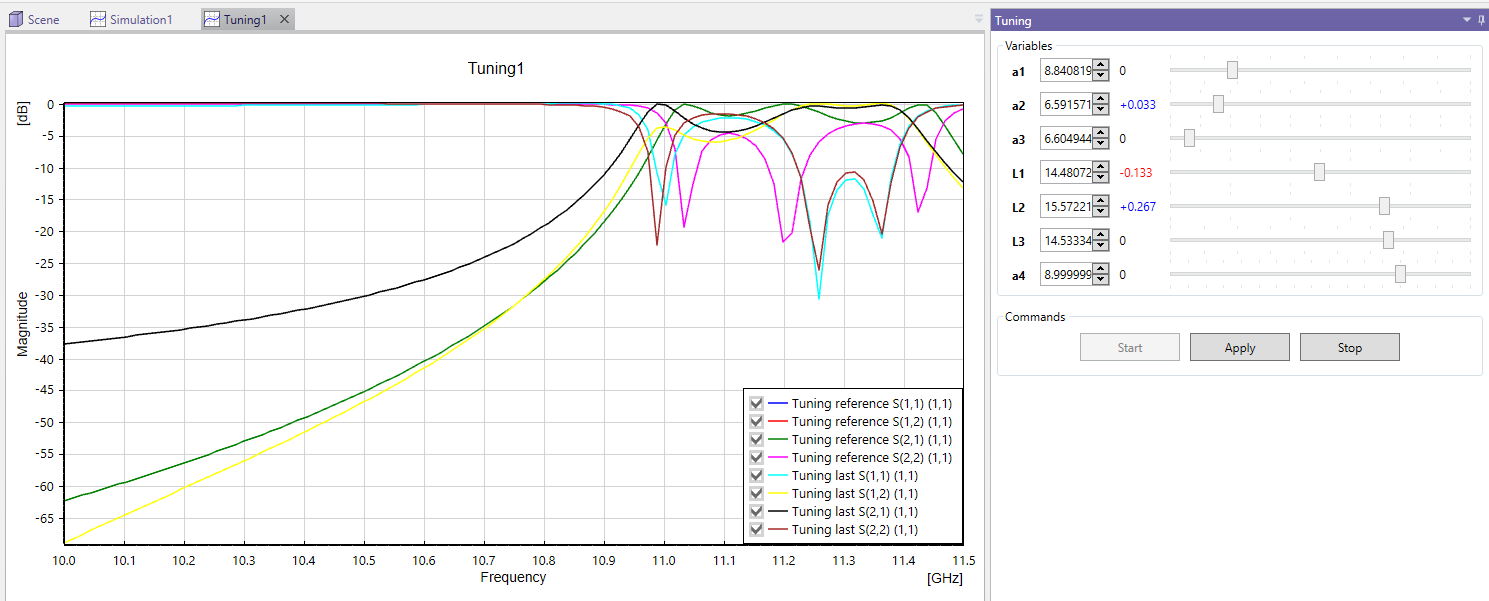
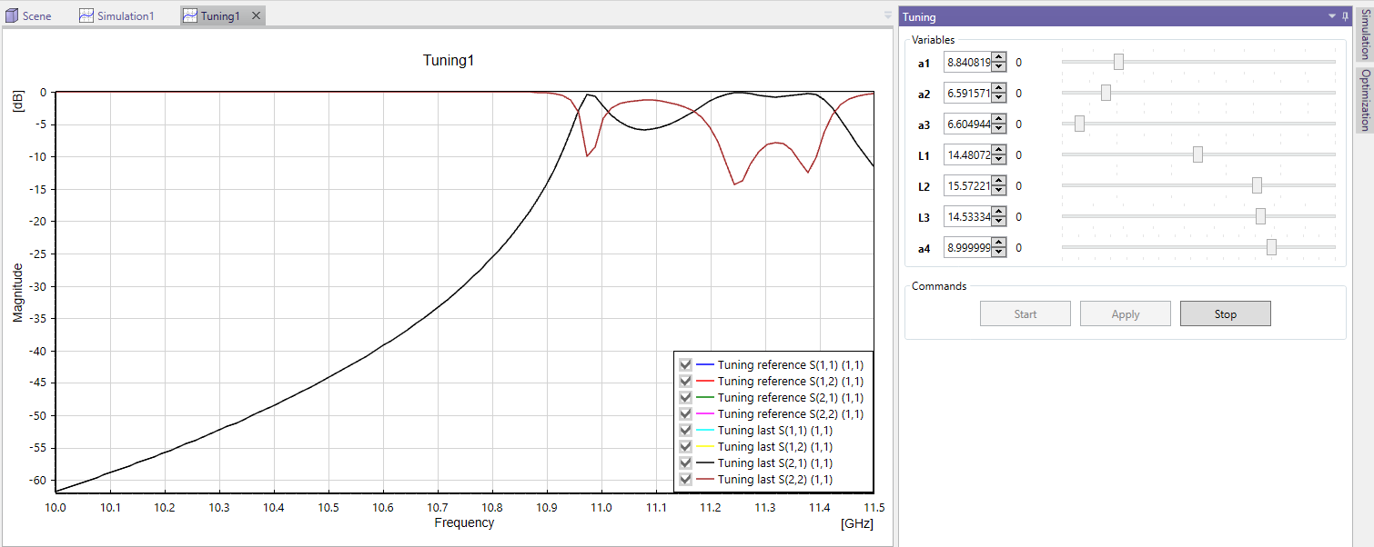
10.2 Standard gradient optimization.
The most fundamental and versatile optimizer available in InventSim is a gradient-based algorithm. In this approach, the user defines the objective function while imposing the requested masks (which specify allowed and restricted regions, defined with inequality operators) on the component’s response. In this context, users can establish multiple objectives based on the frequency domain response of the component undergoing optimization. To add the goal, please right click on the goals list, as shown in Fig.10.5, and then define the goal in a straightforward manner.
Once the goals are set and the optimization variables are defined, the optimization can be started. Please note, that the optimization is allowed only when fast frequency or interpolating sweep is activated.
The optimizer aims to find the best attainable solution but does not guarantee goal achievement. Success depends on various factors, including the definition of the cost function, meshing accuracy and the feasibility of the structure to meet the specified requirements.
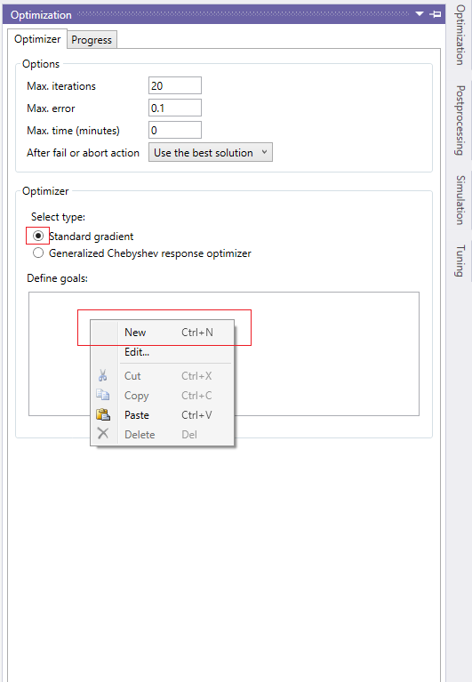
10.3 Generalized Chebyshev Cross-Coupled Filter Optimizer / Coupling matrix synthesis
One of the features of InventSim is a built-in software component for optimization of the RF/microwave coupled resonator filters. With this module, you can easily define the requested filter prototype response by using basic filter specifications such as the passband, insertion, loss level and the positions of transmission zeros (Fig.10.6).

Once the desired response is defined by the user and ready, the goal window can be closed. InventSim will save this response as the reference (goal) for the optimization. If the structure is parameterized with optimization variables, you can start the optimization using the "Optimization" button (Fig.10.7). In order to use the optimization feature, fast frequency sweep must be enabled in the project!
The optimizer is then started. It controls the design in a fully automated manner. The algorithms used during optimization involve a zero-pole cost function that usually exhibits fast convergence when filtering structures are optimized. The response sensitivities are computed using mesh perturbation analysis algorithms implemented in our geometry kernel. To speed up computation, mesh deformation can also be used during the optimization process. The response of each iteration is shown on the plot and plots of optimization progress are available. If optimization is stopped, the best solution is taken as as the current value of design variables. The same tool can be used to perform a coupling matrix synthesis for a provided low-pass filter prototype response. Note, the coupling matrix is not needed to perform design optimization!
In the examples folder, you can find the project file ’wg_optimization.ispr’ which demonstrates the efficiency of the filter optimizer on the example of a rectangular cavity waveguide filter design.
Remarks:
-
• The filter optimizer usually exhibits fast convergence, as long as the response is feasible to achieve in the model.
-
• The optimizer is suited for cross-coupled filter structures for which the response can be described with a rational function. Other filter types, like extracted pole filters, are not supported.
-
• As in every other optimization scheme, the convergence of optimization can not be guaranteed.
10.4 Optimization troubleshooting
A crucial factor for successful design optimization in InventSim is a proper parameterization of the 3D model. To achieve maximum efficiency, the topology of the model (i.e. the number of surfaces and edges, along with their relations) should not change within the tuning/optimization process. This consistency allows for efficient geometry processing and the assessment of design sensitivities. If you encounter errors during optimization, they often stem from unexpected changes in the geometry’s topology or the creation of very small edges or surfaces when altering the design variables. In such cases, we recommend thoroughly inspecting your model and resolving any parameterization issues.
11 COM Interface
One of the features of InventSim is a built-in Component Object Model (COM) interface for inter-process communication. This interface allows other, COM-compatible, processes to communicate with the InventSim software and control the application - i.e. access program data structures and execute procedures. With COM, you can easily connect other application to InventSim and automate the tasks executed within InventSim using commands and custom scripts. COM server is registered by default when installing the InventSim software by using GUID= ’EMIvent.InventSim.App’ (GUID is a unique number that COM uses to identify interface). Several programs support COM technology2, here are some examples: Matlab, GNU Octave, Labview, Python, Visual Basic Script (VBS).
The COM interface of InventSim gives you the options to:
-
• Create, Load, Save projects.
-
• Create, Modify variables.
-
• Create 2D and 3D primitives.
-
• Perform Boolean operations on objects.
-
• Define ports.
-
• Set simulation settings.
-
• Start the simulation and fetch the results.
The reference for the COM interface methods and its properties (API) is described in a separate documentation file ’COM_API_Doc.chm’, stored in InventSim installation folder.
11.1 An example: Connecting/scripting with Matlab\GNU Octave
To start the InventSim COM server from Matlab or GNU Octave, execute the command 3:
App = actxserver('EMInvent.InventSim.App');
The resulting Matlab variable App will be handled to the COM interface of InventSim.4 Using this handle gives you the access to the
fields and methods for objects defined in the COM interface. For example, you might write a simple Matlab script that loads the project file from a specified path on disk, performs the simulation and loads the scattering parameter
\(s_{11}\) into Matlab workspace:
App = actxserver('EMInvent.Simulator.App');
App.ShowWindow(1);
App.OpenProject('C:\h_plane\channel8.ispr');
App.StartSimulation();
while App.IsJobRunning==1
   pause(1);
end
s11 = App.ActiveProject.Simulation.GetResult(0, 1,1,1,1);
3 In GNU Octave, install and load the ’windows’ package first
4 If InventSim is already running, the result will be registered as a handle by the active InventSim window. If InventSim is not open, the InventSim process will be started in the background. To show the InventSim window, invoke App.ShowWindow(1);
11.2 Scripting using Python
To connect to the InventSim COM server from Python (Windows x64 only), the package comptypes needs to be installed5 in Python environment. The script below shows how InventSim COM engine
can be accessed from Python by using the comtypes module:
# IS_connect.py
# script connects to InventSim from Python
import comtypes.client as cc
import comtypes
from cc import CreateObject
App = CreateObject("EMInvent.InventSim.App")
The App is a handle for the instance of InventSim created in Python. You can interact with InventSim by using this handle.
5 To install it, use the default package manager and execute the following command: python -m pip install comtypes. Make sure that pip, setuptools, wheel packages are up to date with the python -m pip install --upgrade pip setuptools wheel command.
11.3 Scripting guide
Several examples of COM scripting are shown in the dedicated COM API guide (Fig.11.1), accessible via the InventSim application from the menu ’Help -> COM API Examples’. The guide shows examples of invoking the COM functions from three environments: C#, Matlab, and Python.
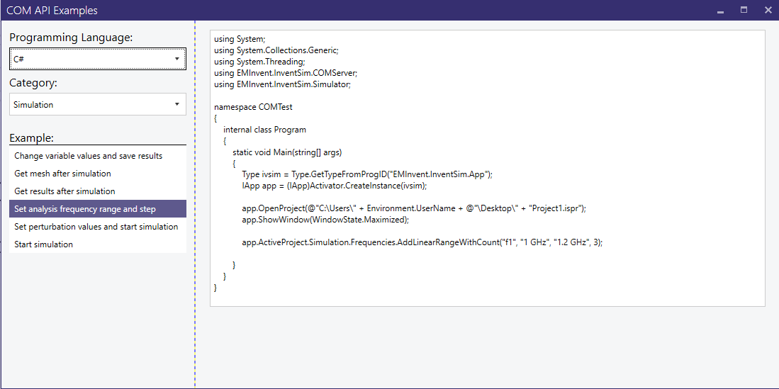
11.4 Command line execution
The solver process can be run directly from the command line. The executable can be found in $InventSim_PATH\simulator\FEMCPP2.exe . To run the simulation, all of the input simulation files,
like mesh and solver options, have to be already generated with InventSim GUI. To re-run the simulation from command line, simply execute:
FEMCPP2.exe project_name
where project_ name is the core-name of all project files (with no file extension). The simulation should start. The results, like the scattering parameters file project_ name.sNp, will be saved in
the project folder.
12 Custom optimization with COM
The methods implemented in InventSim COM interface allow you not only to edit and/or simulate the structure, but also to define your own optimization schemes. The software can be accessed from external tools like Matlab/GNU
Octave where you can easily define a custom optimization goal. If you would like to apply gradient-based optimization routines, like fmincon() or fminimax(), InventSim can provide the responses
(S-parameters) for user-defined perturbations of design parameters (optimization variables). The perturbation can be defined using the following method:
App.ActiveProject.Simulation.SetPerturbationValues(x_pert)
where x_pert is a vector of \(N\) values of perturbed design parameters. If the simulation is run with non-empty vector x_pert, then the solver will also compute the set of \(N\)-responses,
subsequently for each perturbation of design parameters at a time. This set of responses can be accessed with the function:
Sp_ij = App.ActiveProject.Simulation.GetPerturbationResult(q, Port_i, Port_j, Mode1, Mode2)
where \(q=0..N-1\) is the design parameter index (zero-based index), and (Port,Mode) parameters define the row and column of scattering matrix to be extracted. Size of output \(S_p\) confines with number of frequency points defined in the project.
The output vector \(S_p\) can be used, for example, to compute the gradient of S-parameters in frequency domain using finite-difference approach. Please note: to compute the perturbed responses InventSim is only executed once, similar to meshing, which is also done once.
13 Notes on modeling errors
"... Under no circumstances does a competent microwave designer assume that the results of an EM analysis (or of a measurement) are correct. They do not even assume that the results might be wrong. The competent designer assumes the results are in fact wrong, and takes on the job of estimating by just how much the results are wrong..."
James C. Rautio
Microwave De-embedding, 2014
In every computer simulation of physical phenomena, we construct the mathematical model of that phenomena that aims to be as close to the reality as possible. It is still only an approximation. One needs to remember that the outcome of a computer simulation is strongly dependent on the model that was used, its properties and the solution techniques. Therefore, the user should always verify the simulation results and try to estimate how far from reality they might be.
There are several types of errors that influence the outcome of the simulation that a competent user should be aware of [5], two of them are:
-
• Limitations of mathematical models. While the Maxwell equations are a proper description of electromagnetic wave interaction with matter (at least when quantum effects are not included), the models are derived from those equations with some assumptions than you should be aware of. For example, radiation boundary conditions, or lossy conductor boundary conditions, are just approximations of real-life phenomena and have to be used with care. The recommended solution is to validate the mathematical model with prototype measurements.
-
• Discretization. When solving the electromagnetic problem with FEM, the fields inside the domain are approximated using base functions. The number of base functions used (or mesh density) strongly influences the results of simulation and it is model dependent. In theory, when the mesh is refined, the results should converge to a "real" solution. In reality, it is hard to determine if the current mesh is dense enough. Therefore, even the application of adaptive mesh refinement does not guarantee the convergence of the solution.
However, errors of the simulation are not the only problem that can be encountered. Even if the simulation is exact, there is still a risk of encountering manufacturing tolerance errors when manufacturing the device. The resulting prototype would then be slightly different from the computer model. Therefore, you should always look for the compromise between simulation accuracy and manufacturing accuracy during the design phase.
14 Useful keyboard shortcut keys
| Key | Shortcut description |
| O | Pick objects |
| F | Pick faces |
| E | Pick edges |
| Ctrl + T | Find SimObject |
| Shift | Keep objects during Boolean operations |
| Shift + Enter | Finish 2D polygon |
14.1 Troubleshooting
14.1.1 Resetting the widow layout
In order to restore the default window layout, you can:
-
• use the "Reset window layout" icon in "View".
15 Changelog
-
• Version 5.1.12
-
– Top new fixed:
-
* Fixed an issue that caused Perturbation Analysis to fail during optimization.
-
* Fixed an issue that caused incorrect boundary conditions to be set when a dielectric element was placed inside a PEC element.
-
* Fixed an issue that caused incorrect coordinate system activation.
-
-
-
• Version 5.1.11
-
– Top new fixed:
-
* Fixed an issue that caused scene not to initialize.
-
-
– Top new added:
-
* Added the possibility to export variable data to CSV files.
-
-
-
• Version 5.1.10
-
– Top new fixed:
-
* Fixed an issue that caused the application to crash when right-clicking on an object’s material.
-
* Fixed an issue that caused an error message when editing imported plot series.
-
* Fixed a rare issue that caused an error when applying the Extrude Ruled operation.
-
* Fixed issues that caused incorrect window positioning on high-DPI screens.
-
* Fixed an issue where the last-used optimizer was not selected after loading a project.
-
-
-
• Version 5.1.9
-
– Top new fixed:
-
* Fixed a rare issue that caused the Standard Optimizer to stop due to a null reference error.
-
* Fixed an issue that caused an error when loading a project with imported plot series.
-
-
-
• Version 5.1.8
-
– Top new fixed:
-
* Fixed an issue that caused an incorrect variable expression to be set after renaming a variable.
-
* Fixed an issue that caused errors when manipulating mesh deformations via COM in MATLAB.
-
-
-
• Version 5.1.7
-
– Top new fixed:
-
* Fixed an issue casing the application to crash on exiting.
-
-
– Top new added:
-
* Added an improved warning message for waveguide port cutoff frequency, indicating which port the message refers to.
-
-
-
• Version 5.1.6
-
– Top new fixed:
-
* Fixed an issue that allowed the coordinate system used in postprocessing tasks to be removed.
-
* Fixed an issue that caused an incorrect error message to be shown after entering an invalid RLC element value.
-
* Fixed issues that caused errors when working with projects having paths longer than 260 characters.
-
* Fixed rendering issues when not using Advanced Renderer option.
-
* Fixed an issue that caused duplicate files to appear in the recent projects list.
-
-
– Top new features:
-
* Added the ability to import and export plot series to and from CSV files.
-
* Added new datasets to the radiation solution: Gain and Axial Ratio.
-
* Added a plot operator for effective conductivity (“sigma”).
-
* Added Advanced Meshing parameters.
-
-
– Top improvements:
-
* Significantly improved variable management performance when handling hundreds of variables.
-
-
-
• Version 5.1.5
-
– Top new fixed:
-
* Fixed an issue that caused incorrect preprocessing results.
-
* Fixed an issue where the STL ASCII format was missing the "vertex" keyword.
-
* Fixed an issue that caused the application to crash when manipulating the mesh deformation positions list.
-
-
– Top new added:
-
* Added Line Calculator plugin.
-
* Added Interdigital Filters plugin.
-
* Added Circular Spiral Inductors plugin.
-
* Added Rectangular Spiral Inductors plugin.
-
* Added Polygonal Spiral Inductors plugin.
-
* Added Parallel Coupling Bandpass Filters plugin.
-
* Added the ability to move variables up and down in the variable list.
-
* Added the ability to expand/collapse entire coordinate systems tree.
-
-
– Top improvements:
-
* Improved preprocessing performance and stability.
-
* Improved GUI responsiveness when selecting objects with complex boolean operations.
-
* Changed Perturbation Analysis to use only performance cores on modern Intel CPUs, improving performance.
-
* Added more comprehensive error messages in case of meshing failures.
-
* Improved optimization convergence by modifying initial step length calculation.
-
-
-
• Version 5.1.4
-
– Top new fixed:
-
* Fixed an issue causing, in some cases, TEM mode ports to have an incorrect impedance calculation.
-
-
-
• Version 5.1.3
-
– Top new fixed:
-
* Fixed an issue that caused a new mesh deformation parameter to be added incorrectly.
-
* Fixed an issue that caused an inconvenience when entering negative values for optimization goals.
-
* Fixed an issue that caused application crash when clicking on mesh deformation parameter list.
-
-
-
• Version 5.1.2
-
– Top added:
-
* Boundary condition object list edit functionality.
-
-
– Top new fixed:
-
* Fixed an issue that caused projects to fail to open when a material parameter was assigned a variable with specific values.
-
* Fixed an issue that caused undoing of MakeFillet operation result in an incorrect shape.
-
* Fixed an issue that caused application to crash when clicking on certain messages.
-
-
-
• Version 5.1.1
-
– Top new fixed:
-
* Fixed an issue that caused unnecessary error message to appear in certain situations related to lumped ports.
-
* Fixed an issue that caused port visualization not be shown.
-
* Fixed an issue that caused incorrect helix shape be created.
-
-
-
• Version 5.1.0
-
– Top new:
-
* Added support for drawing helices (Section Helix).
-
* Added support for exporting 2D geometry to DXF files.
-
* Added plugins for creating planar inductors.
-
* Vastly improved performance of mesh deformations.
-
-
– COM API changes:
-
* Added API to mesh deformations feature.
-
* Added IApp.Release() method to release COM connection to the server.
-
-
-
• Version 5.0.0:
-
– Top new:
-
* Added Boundary conditions visualization to inspect how boundary conditions are set in the project (Section "Boundary conditions visualization").
-
* Added cut view to the scene rendering (Section "Cut view").
-
* Changed variables view to a form of table for better variables management and manipulation (Section "Variables and equations").
-
* Variable snapshots (Section "Variable snapshots").
-
* Any operation can now be deleted, not only the last one.
-
* Introduced combined shape deformations giving more flexibility (Section "Shape deformations").
-
* Added COM API examples browser.
-
* Tuning ranges have been limited to provide more accurate results.
-
-
-
• Version 4.0.8:
-
– Top new added:
-
* Boundary conditions can now be disabled.
-
-
– Top new fixed:
-
* Fixed issues causing mesh deformation to fail.
-
-
-
• Version 4.0.7:
-
– Top new features:
-
* Export plot series to CSV files.
-
-
-
• Version 4.0.6:
-
– Top issues fixed:
-
* Fixed several meshing issues.
-
* Fixed performance lags when changing variable values.
-
-
– COM API changes:
-
* Added new method IObjects.MakeFace() for creating faces out of closed set of edges.
-
-
-
• Version 4.0.5:
-
– Top new features:
-
* Tuning performance has been improved.
-
-
– Top issues fixed:
-
* Fixed issue that caused error when using ExtrudeRuled tool.
-
* Fixed issue that caused application to crash occasionally when using boolean tools.
-
* Fixed issue that caused projects with lumped ports to show incorrect admittance and impedance parameters.
-
-
– COM API changes:
-
* COM API examples have been added.
-
* Added new method ITuning.GetResult() for obtaining tuning results.
-
-
-
• Version 4.0.4:
-
– Top issues fixed:
-
* Fixed issue that caused error when using ExtrudeRuled tool.
-
* Fixed issue that caused application to crash occasionally when using boolean tools.
-
-
-
• Version 4.0.3:
-
– Top new features:
-
* Cylinder and Cone plane (axis) can now be changed after their creation.
-
* Variable used in equations are no longer required to precede the equations thus variables can be sorted in any order.
-
-
– Top issues fixed:
-
* Fixed issue when a project had inconsistent variable values when optimization failed.
-
* Fixed issues that caused incorrect scene rendering on high DPI screens.
-
-
– COM API changes:
-
* Added new methods ISimObject.GetFacesAt2(), ISimObject.GetEdgesAt2() and ISimObject.GetFaceEdges2() returning a new interface ISimObjectCollection representing a collection of ISimObject objects instead of an array. Those methods are preferred when using MATLAB as the COM client.
-
* Added new methods IObjects.MakeFillet2() and IObjcets.MakeChamfer2() accepting ISimObjectCollection containing edges instead of an array. Those methods are preferred when using MATLAB as the COM client.
-
* Added a new method IMeshRefinements.AddMeshRefinement2() accepting ISimObjectCollection containing objects instead of an array. This method is preferred when using MATLAB as the COM client.
-
-
-
• Version 4.0.1:
-
– Top new features:
-
* Search box and refresh button added to open file dialog.
-
-
– Top issues fixed:
-
* Fixed issues with simulation of projects having name consisting of particular non-Latin characters.
-
-
-
• Version 4.0.0:
-
– Top new features:
-
* New field visualization capabilities including isosurfaces and isolines rendering for scalar fields visualization, as well as reworked vector field rendering. For more information please refer to section 9.3.
-
* Reworked copy/paste mechanism allowing versatile copying between projects taking into account relations between SimObjects, variables and coordinate systems.
-
* Port reference plane shift has been added.
-
* A new tool ExtrudeAlongPath has been added which allows to make
-
* Fillets and chamfers now works also for 1D objects i.e. curves.
-
* Far field distance can now be specified for far field calculation.
-
-
– Top issues fixed:
-
* Performance of preprocessing stage of simulation has been vastly improved.
-
* Stability of meshing has been improved.
-
* Application was crashing during tuning when analytic port coordinate system was incorrectly parameterized.
-
* Application was crashing when SimObjects visibility was changed during simulation.
-
* Fillets and chamfers were incorrectly added to objects if edges from several different SimObjects were selected.
-
-
– Other changes:
-
* SimObject visibility can now be changed for many objects at once.
-
* Fillets and chamfers can now be added for multiple edges owned by different SimObjects at once.
-
* Mesh visualization can now be added before meshing.
-
* During optimization, best iteration is now saved in optimization best solution folder.
-
* Adaptive meshing error plot has been added.
-
-
– COM API changes:
-
* Added IVariable.SetValues method to allow setting variable value, minimum and maximum values using one function call.
-
* Added IMesherParameters interface to allow control over meshing parameters. It can be accessed via ISimulation.MesherParameters property.
-
* Added IAdaptiveMeshing interface to allow control over adaptive meshing process. It can be accessed via IMesherParameters.AdaptiveMeshing property.
-
* Added IMesh interface providing access to a mesh. Current mesh can be obtained via new ISimulation.GetMesh method.
-
* Method ISimulation.GetMeshMorphingData renamed to GetMorphedMesh. The method now returns the morphed mesh via IMesh interface.
-
* Property ISimulation.OverrideMeshFile renamed to OverrrideMesh and now is of IMesh type.
-
* Method ISimulation.ClearPertubationValues renamed to ClearPerturbationValues (grammar error corrected).
-
* Added IVariable.SetValues method to set minimum and maximum values of variable using one function call.
-
-
-
• Version 3.0.3:
-
– Top issues fixed:
-
* Optimization goals were sometimes incorrectly loaded from project file.
-
* Application was crashing when objects were modified and analytical ports were defined.
-
-
-
• Version 3.0.2:
-
– Top new features:
-
* Fillets and chamfers can now be added for multiple edges owned be different SimObjects at once.
-
-
– Top issues fixed:
-
* Application was crashing during tuning when analytic port coordinate system was incorrectly parameterized.
-
* Fillets and chamfers were incorrectly added to objects if edges from several different SimObjects were selected.
-
-
-
• Version 3.0.1:
-
– Top new features:
-
* Added mesh export to STL file.
-
-
– Top issues fixed:
-
* Fixed some memory leaks.
-
* Object were not selected correctly in orthographic camera mode.
-
* Error message was being shown on rare occasions during boolean operations.
-
* Delete solution button was not active.
-
* User could add a postprocessing task with an already existing name.
-
-
-
• Version 3.0.0:
-
– Top new features:
-
* Plot series definition window has been improved and now supports the equation-based data (scripts), including multiple math functions and operators including field normalization,
-
* VSWR and Group delay have been added to simulation data sets,
-
* Standard Optimizer goals definition interface has been improved and now supports the equation-based goals that utilize multiple math functions and operators,
-
* 3D object deformation via Shape-Deformation engine has been added which allows to simulate geometries not available when using CSG approach (requires a separate license)
-
* Autocomplete functionality has been added to text input fields which provide users variable suggestions allowing quick typing of expressions,
-
* Boolean operations operands can now be viewed when selected allowing better analysis of complex geometries,
-
* Scene rendering engine has been improved providing anti-aliased image and better visuals of opaque objects,
-
* Importing geometry from OpenCascade BREP files has been added,
-
* Oersted unit (Oe) has been added for convenient definition of gyromagnetic materials,
-
* Design sensitivities plot has been added in the optimization panel improving control of the optimization process.
-
-
– Top changes:
-
* A new project file format has been introduced to accommodate new functionalities of plot series and optimization goals definition. Projects saved in version 3 are not compatible with earlier versions of InventSim.
-
-
– Top issues fixed:
-
* Application was crashing when extrusion draft angle was set to a positive value,
-
* Smith and polar charts were showing incorrect results.
-
-
– COM API changes:
-
* IApp.StartSimulation(IProject) method has been added allowing starting optimization,
-
* IMessages.GetCount() and IMessages.GetCount(MessageStatus) methods have been added,
-
* IMeshRefinements renamed to IMeshOperations,
-
* IMeshRefinement renamed to IMeshOperation.
-
-
– Known issues:
-
* When optimization finishes, simulation plots are not automatically updated - simulation has to be performed after optimization in order to show correct results,
-
* Simulation using Fast frequency sweep with iterative solver can sometimes return error - Interpolating sweep can be used instead.
-
-
16 Acknowledgements
Selected components of IventSim software were developed under support of the Foundation for Polish Science within the TEAM-TECH Program, cofinanced by the European Regional Development Fund, Smart Growth Operational Program 2014 - 2020 (project EDISOn: Electromagnetic Design of fexIble SensOrs), under agreement POIR.04.04.00-00-1DC3/16-00.
EULA
InventSim End-User Software License Agreement (EULA)
Licensor: EM Invent sp. z o.o., Trzy Lipy 3, 80-172, Gdansk, Poland
This End-User License Agreement (hereinafter ’Agreement’) is a legal contract between you, as either an individual or an Entity (hereinafter ’End User’ or ’Licensee’), and EM Invent sp.z o.o. (hereinafter ’EM Invent’ or ’Licensor’). By accepting this End User License Agreement (EULA) or by downloading or using the Software you signify that you have read and agree to all the terms of this license agreement.
Preliminary Statements
The licensor holds as proprietor and authorized agent the software copyright for the product InventSim - a 3D FEM Electromagnetic Simulation and Optimization Framework (hereinafter ’Software’). All industrial property rights to the Software delivered by EM Invent, and in particular the comprehensive copyright, together with all rights in the Software, documents and information provided as part of the preparatory phase of the Agreement and during its performance (including warranty and maintenance) shall remain with EM Invent and its licensor.
Software versions and License types
The Software is distributed in two versions: i) Full version with all functionality available and ii) Demo (or Lite) version with limited functionality.
The Software in Demo mode (or Lite version) is a free evaluation version of the Software that does not include the full functionality found in the full version. The Software in Demo/Lite version is provided ’as-is’ and EM Invent provides no support for the Demo version. The Software in Demo mode is made available to you for the purpose of demonstrating the program capabilities of the software so you can evaluate whether to purchase a full license of the software. Demo version can be used for educational and/or commercial activities, but without any warranty and on your own risk.
The Software in Full version is available in the following license types:
-
• Evaluation License: The Software may be used only for purposes of internal evaluation and demonstration of the capabilities of the Software. The Software may not be used to generate any work product that will be used in any Commercial manner.
-
• Education License: The Software may be used only for: (A) purposes directly related to learning, teaching, training and research that are part of the instructional functions performed by a formal educational institution, such as a degree-granting or certificate-granting college or university, or any other dedicated learning, teaching or training facility; or (B) training and education purposes by a Licensee engaged in Commercial activities. The Software may not be used to generate any work product that will be used in any Commercial manner.
-
• Commercial License: The Software may be used for Commercial or non-Commercial purposes.
The aforementioned license types are available either as perpetual license or time-limited license.
License Grant
The End User has, subject to the terms and conditions of this EULA, a non-exclusive license (’License’), to use the Software in object code format, solely for End User’s internal business purposes for the management and processing of its own data and not the data of any third party(ies). License is perpetual, unless the Software is delivered to End User as part of a Transaction on a non-perpetual basis for a defined period, rented or delivered for testing purposes, in such case, the End User’s right to use such Software will cease on the end date of the defined period.
The Software is provided to the End User for its own, internal use only. The End User is not permitted to hire out the Software in whole or in part, in whatsoever form or for whatsoever purpose. The End User shall not lend the Software, in whole or in part. The Licenses under these EULA are granted subject to the condition that the Software is operated by End User itself and not by any third parties. Prior to transferring the operation of the Software to the respective third party, End User shall be required to enter into the necessary written agreement with EM Invent.
EM Invent provides the End User with the software license key and/or USB dongle necessary to run the Software in Full version and verify the valid license. The End User shall ensure that the program key and the dongle are kept in a safe place. The End User bears the risk of dongle loss (including through theft and other forms of loss). If the dongle is lost, the End User shall purchase a new copy of the Software if it wants to continue to use the Software in accordance with the contract.
Restricted warranty
The licensor is not liable for damage or subsequent damage which the software causes to the licensee or a third party directly or indirectly. The licensor is not liable for certain performance results obtained by the licensed software. This also applies to the working order of the software for the agreed or other purposes. The licensee bears the risk of the economic utility. The licensee will inform the licensor about occurring quality defects provided they are based on technical software faults or if they are due to defective management of the programming tasks. The licensor will promptly transmit, on demand, all the necessary information and documents to eliminate any defects.
As far as permitted by law the licensor in regard to the software and the accompanying written documents declines any further warranties regardless of the fact if they were granted explicitly or tacitly, he also explicitly declines warranty for the usage and fitness for a certain purpose.
As far as permitted by law the liability for damage of any kind will be excluded as agreed. This includes direct and/or indirect damage from lost profits, operating trouble, or any other property loss or physical injury.
License for third party software
EM Invent has been granted licenses to distribute certain third party software. As a condition of those licenses, EM Invent is required to distribute the software subject to specific terms and conditions, which may be different from or additional to those contained herein for Software. Licensee understands and agrees that acceptance of this agreement also confirms Licensee’s acceptance of the applicable provisions for use, including the restrictions on use, of such third party software. Licensee may contact EM Invent to obtain the current applicable provisions. Licensee’s breach of the applicable provisions of any third party’s license terms shall also be considered a material breach of this Agreement.
EM Invent is explicitly excluded from all liability for damages of any kind which might be caused by any third party software with the Software. Additionally EM Invent is excluded from any obligation to provide remedial actions for damages of any kind which might be caused by any third party software.
Maintenance and Support
For the Full version of the Software EM Invent can provide to the Licensee software maintenance and support services, namely (i) making available to the Customer patches, fixes, updates and/or enhancements generally made available to customers from time to time, if any, and (ii) technical support, on an as-needed basis for the sole purpose of responding within a reasonable period of time and attempting to address technical issues relating to the use of the Software. This may include online technical support and telephone support. The support and maintenance services are provided by EM Invent only if a separate Maintenance and Support fees are paid by the Licensee.
Without limiting the generality of the foregoing, any requests by the Customer for additional features or functionality that fall outside of InventSim ongoing updates and/or enhancements of the Software are excluded from Maintenance and Support Services.
Usefulness clause
It is not possible to achieve useful results for practical purposes with the InventSim unless they are subjected to separate procedures in which all data are verified, tested and checked. In particular no product shall be constructed with the results obtained with the InventSim which have not been submitted to other known procedures of inspection, construction and subsequent tests of the product. The beta/Demo/Lite version of InventSim is only for testing the software and its capabilities. It should not never be used for designs that are going into production.
Infringements
EM Invent will not be held liable for any patent infringements committed by the end user as a result of the end user’s design, production, offer or distribution of patent protected components or structures created using the software covered by this contract. This Disclaimer refers in particular to infringements of Third Party Intellectual Property Rights.
Benchmarking
The EULA does not prevent End User from using the Software for internal benchmarking purposes. However, End User shall treat any and all benchmarking data relating to the Software, and any other results of your use or testing of the Software which are indicative of its performance, reliability or quality, as confidential information and you shall not disclose such information to any third party without the express written permission of EM Invent.
Export restriction
The Software and Documentation, including a third part software used, might be further subject to United States and European Union export controls. No software or Documentation may be Provided or otherwise exported or re-exported (1) into (or to a national or resident of) Cuba, Iran, Iraq, Libya, North Korea, Sudan, Syria, or any other country to which the United States or EU has embargoed goods; or (2) to anyone on the U.S. Treasury Department’s list of Specially Designated Nationals or the U.S. Commerce Department’s Table of Deny Orders. By Installing or using the Software or Documentation, you represent and warrant that you are not located in, under the control of, or a national or resident of any such country or on any such list.
Reverse engineering
Modification, reverse engineering, reverse compiling, or disassembly of the Software is expressly prohibited. If, however, you are a resident of the European Union (’EU’), information necessary to achieve interoperability of the Software with other programs within the meaning of the EU Directive on the Legal Protection of Computer Programs will be available to you from EM Invent upon written request.
Jurisdiction
This agreement is subject to the law of Poland. Place of jurisdiction is Gdansk (Poland).
References
-
[1] J. Jin, "The Finite Element Method in Electromagnetics," John Wiley and Sons Inc., New York, 2002
-
[2] J. Jin and D.J. Riley, "Finite Element Analysis of Antennas and Arrays," John Wiley and Sons Inc., New Jersey, 2009
-
[3] Y. Zhu and A.C. Cangelaris, "Multigrid Finite Element Methods for Electromagnetic Field Modeling," IEEE Press - Wiley Interscience, John Wiley and Sons, NJ, 2006
-
[4] J.L. Volakis, A. Chatterjee and L.C. Kempel, "Finite Element Method for Electromagnetics. Antennas, Microwave Circuits and Scattering Applications," IEEE Series on Electromagnetic Wave Theory, IEEE Press, NJ, 1998
-
[5] D.B. Davidson, "Computational Electromagnetics for RF and Microwave Engineering," Cambridge University Press, 2 edition, Nov. 2010
-
[6] G. Pelosi, R. Coccioli and S. Selleri, "Quick Finite Elements for Electromagnetic Waves," Artech House Inc., 2009
-
[7] P. Ingelstrom, "A New Set of H(curl)-Conforming Hierarchical Basis Functions for Tetrahedral Meshes," IEEE Transactions on Microwave Theory and Techniques, Vol. 54, Jan. 2006
-
[8] J.P. Swartz and D.B. Davidson, "Curvilinear Vector Finite Elements Using a Set of Hierarchical Basis Functions," IEEE Transactions on Antennas and Propagation, Vol. 55, Feb. 2007
-
[9] J. Rubio, J. Arroyo and J. Zapata, "Analysis of Passive Microwave Circuits by Using a Hybrid 2-D and 3-D Finite Element Mode-Matching Method," IEEE Transactions on Microwave Theory and Techniques, Vol. 47, Sept. 1999
-
[10] M. Eguchi and M. Koshiba, "Accurate Finite-Element Analysis of Dual-Mode Highly Eliptical-Core Fibers," Journal of Lightwave Technology, Vol. 12, April 1994
-
[11] M. Koshiba, Y. de Tsuji, "Curvilinear Hybrid Edge/Nodal Elements with Triangular Shape for Guided-Wave Problems," Journal of Lightwave Technology, Vol. 18, pp.737-743, May 2000
-
[12] J. Schöberl, "NETGEN An advancing front 2D/3D-mesh generator based on abstract rules," Computing and Visualization in Science, Vol. 1, pp.41-52, July 1997
-
[15] A. Dziekonski, A. Lamecki and M.Mrozowski, " GPU Acceleration of Multilevel Solvers for Analysis of Microwave Components With Finite Element Method ," IEEE Microwave and Wireless Components Letters, pp. 1-3, Vol.21, Jan. 2011
-
[16] A. Dziekonski, A. Lamecki and M. Mrozowski, "Tuning a Hybrid GPU-CPU V-Cycle Multilevel Preconditioner for Solving Large Real and Complex Systems of FEM Equations," Antennas and Wireless Propagation Letters, IEEE , vol.10, no., pp.619-622, 2011
-
[17] Y. Zhu, A.C. Cangelaris, "Hierarchical Multilevel Potential Preconditioner for Fast Finite Element Analysis of Microwave Devices," IEEE Transactions on Microwave Theory and Techniques, Vol. 50, Aug. 2002
-
[18] P. Nickel, V. Hill, P. Ingelstrom and R. Dyczij-Edlinger, "Multilevel Analysis of Electromagnetic Resonators Using Hierarchical p-Type Finite Elements," 12th Biennial on Electromagnetic Field Computation, Jun. 2006
-
[19] E.Lezar, D.B. Davidson, "Implementation of Arbitrary High Order Hierarchical Vector Basis Functions for Finite Element Analysis of Rectangular Waveguide," 8th IEEE AFRICON Conference - AFRICON’07, Windhoek, Namibia, September 2007
-
[20] J.-S. Wang and N. Ida, "Eigenvalue Analysis in Electromagnetic Cavities Using Divergence Free Finite Elements," IEEE Transactions on Magnetics, Vol. 27, Sept. 1991
-
[21] C.J. Reddy, M.D. Deshpande, C.R. Cockrell and F.B. Beck, "Finite Element Method for Eigenvalue Problems in Electromagnetics," NASA Technical Paper 3485, Dec. 1994
-
[24] A. Kucharski, P. Slobodzian, "The application of macromodels to the analysis of a dielectric resonator antenna excited by a cavity backed slot," 38th European Microwave Conference, EuMC 2008, pp. 519-522, Oct. 27-31, 2008.
-
[25] Robert E. Collin, "Foundations for Microwave Engineering - 2nd edition [Hardcover]," IEEE Press Series on Electromagnetic Wave Theory, 2001
-
[26] Montejo-Garai, J. R. and Zapata, J., "Full-wave design of dual-band double-septum circular waveguide polarizers," Microw. Opt. Technol. Lett., Vol.20, pp. 99–103, 1999
-
[27] C. A. Balanis, "Advanced Engineering Electromagnetics," Wiley, 1989
-
[28] A. Lamecki, "A Mesh Deformation Technique Based on Solid Mechanics for Parametric Analysis of High-Frequency Devices With 3-D FEM," in IEEE Transactions on Microwave Theory and Techniques, vol. 64, no. 11, pp. 3400-3408, Nov. 2016.
-
[29] D. Forti, G. Rozza, "Efficient geometrical parametrisation techniques of interfaces for reduced-order modelling: application to fluid-structure interaction coupling problems", International Journal of Computational Fluid Dynamics, vol. 28, no. 3-4, pp. 158-169, 2014.
-
[30] Z. Levi, D. Levin, "Shape Deformation via Interior RBF", IEEE Transactions on Visualization and Computer Graphics, vol. 20, no. 7, pp. 1062-1075, July 2014.
-
[31] A. de Boer, M.S. van der Schoot, H. Bijl, "Mesh deformation based on radial basis function interpolation", Computers & Structures, vol. 85, no. 11, pp. 784-795, June 2007.
-
[32] M. Botsch, L. Kobbelt, "Real-Time Shape Editing using Radial Basis Functions", Computer Graphics Forum, vol. 24, no. 3, pp. 611-621, Sept. 2005.
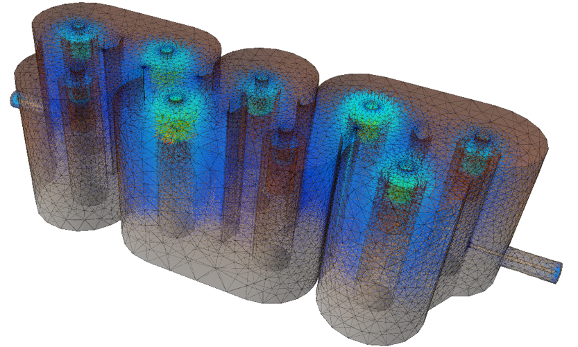

©2021 EM I NVENT SP. Z O. O. (LTD.)
T RZY L IPY 3, 80-172 G DANSK , P OLAND