4 Boundary conditions

One of the fundamental prerequisites needed to get accurate simulation results is the enforcement of proper boundary conditions within the structure. InventSim supports a few types of boundary conditions that can be enforced for a provided surface. (2D object with infinitesimal thickness).

If the results of the simulation do not agree with the predictions, please verify if all the boundary conditions are properly assigned. You can preview the boundary conditions by using the context menu on a 3D scene view window and selecting ’Show boundary conditions.’ The internal part of the structure can be observed with the 3D view cut-plane option available via the main ribbon in the ’View’ section.

4.1 Perfect electric conductor

Perfect electric conductor (PEC) is an artificial condition used to model material with zero resistivity. Practically, it enforces the zero of tangential electric field on that surface:

\begin{equation} \hat {n} \times \textbf {E} = 0 \end{equation}

where \(\hat {n}\) is the unit vector normal to the surface.

The PEC condition is a default boundary at the outer surfaces of the 3D model!

4.2 Perfect magnetic conductor / Natural boundary

Perfect magnetic conductor (PMC) is an artificial condition used to model the material with infinite resistivity. It enforces the zero of tangential magnetic field on that surface:

\begin{equation} \hat {n} \times \textbf {H} = 0 \end{equation}

In result, there will be no electric current at the surface, and the effective conductivity is zero. This boundary condition works as intended as long as it is defined on the outer surface of the structure. If we define the PMC for an internal boundary, then it is transparent for the electromagnetic field, just as the surface on the boundary between two dielectric materials (natural boundary).

4.3 Lossy conductor surface

Surfaces marked as lossy conductors are modeled as infinite, thick surfaces with imposed first order impedance boundary conditions corresponding to the surface impedance of a conductor with finite conductivity \(\sigma \):

\begin{equation} \textbf {E} \times \hat {n} = Z_m \cdot \hat {n} \times (\hat {n} \times \textbf {H} ) \end{equation}

where conductor surface impedance \(Z_m\) is defined as

\begin{equation} Z_m = \frac {1+j}{\sigma \cdot \delta _s} \end{equation}

This model is valid if the radius of surface curvature is large enough compared to skin depth \(\delta _s\). In this case, we assume the current does not penetrate the volume of the conductor, only flows directly on its surface. The model can accurately model real-life scenarios of lossy conductors working in frequencies up to tens of GHz.

4.4 Lumped RLC circuit

InventSim allows one to define a rectangular 2D surface object as a two-port device that represents a parallel or series RLC circuit. To model an RLC circuit impedance boundary condition is applied. At least one value of R,L,C provided by the user must be non-zero.

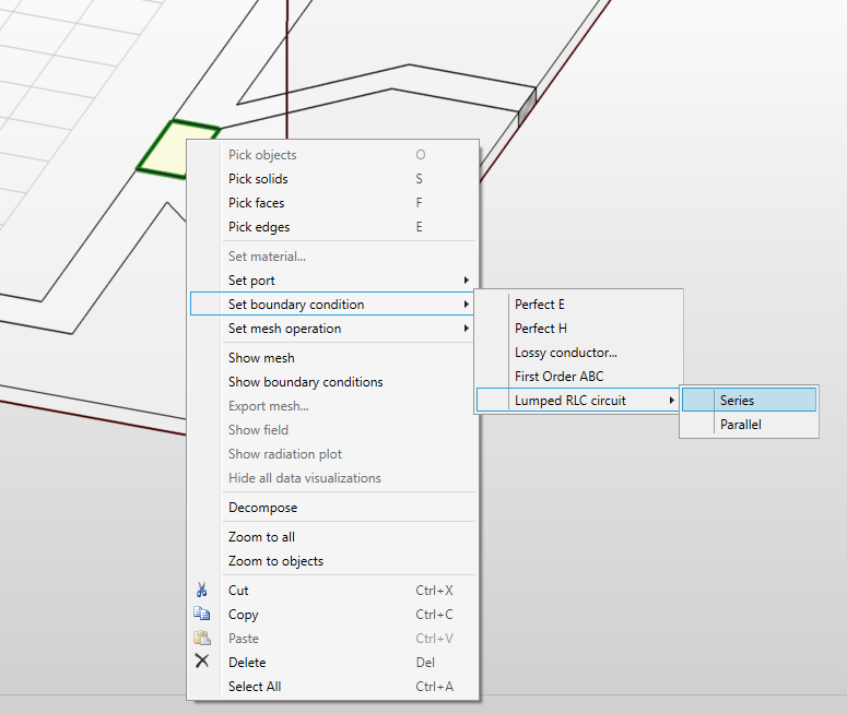
To define the 2D rectangle as an RLC element you need to select the object, invoke the context menu (with right-click) and select the option ’Set boundary condition -> Lumped RLC circuit -> Series Parallel.’ (Fig.4.1). Then we define which pair of opposite edges are element connectors and define the values of resistance R, inductance L, and capacitance C.

4.5 Absorbing boundary condition

In order to truncate the mesh and simulate the infinite free-space environment needed, for example, in antenna applications, an artificial surface that absorbs radiated field should be used. With InventSim, you can introduce an absorbing boundary condition (ABC) that absorbs the incident waves and minimizes reflections from the surface [2]:

\begin{equation} \hat {n} \times (\nabla \times \textbf {E}) + j k_0 \hat {n} \times ( \hat {n} \times \textbf {E}) = 0 \end{equation}

This type of absorbing boundary condition is most efficient when a plane wave direction is perpendicular to the surface and, in the case of incident, at an angle large enough to the surface so that a significant reflection can be observed. In most cases, the recommended minimum distance between the surface and the source of radiation is one-half wavelength. The advantage of using such absorbing boundary condition is the simplicity of its definition on one or several surfaces, including non-planar ones.

When simulating radiating elements, we utilize the fields gathered from radiation boundaries to assess key radiation parameters such as pattern, radiation efficiency, or gain.

4.6 Symmetry planes

The symmetry of the structure can be exploited to reduce the numerical cost of simulation. It can be done by simply cutting the structure in the symmetry plane and enforcing a proper boundary condition.

In InventSim, both PEC and PMC walls can be used as the symmetry planes. The choice to use the symmetry plane and which kind (PEC, PMC) is dependent on the structure and the properties of electromagnetic field solution within the structure, and it requires proper knowledge and experience of the user. In general we:

• • use PEC where the magnetic field is symmetric and electric field is asymmetric.

• • use PMC where the electric field is symmetric and magnetic field is asymmetric.

4.6.1 Example

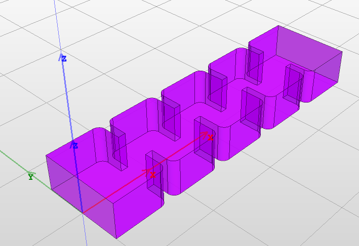
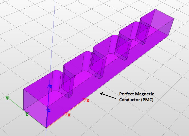
The application of symmetry planes can be shown in an example of the H-plane waveguide filter simulation. The 3D view of the structure is shown in Fig. 4.2. One can notice that the structure is symmetric with respect to XZ-plane. Only \(TE_{n0}\) modes (with \(n=1,3,5...\)) are excited within the structure. The electric field is symmetric along the symmetry plane and all modes have a maximum of the electric field (and zero magnetic field) in the symmetry plane. Therefore, instead of simulating the whole structure, you can cut a half of it (Fig.4.3), and define the surface on symmetry plane as a perfect magnetic conductor.

The port can be added now - InventSim will calculate the mode templates that take the symmetry into account. In result, you can reduce the problem size by half while preserving the accuracy of the simulation at the same time.

4.7 Boundary conditions visualization

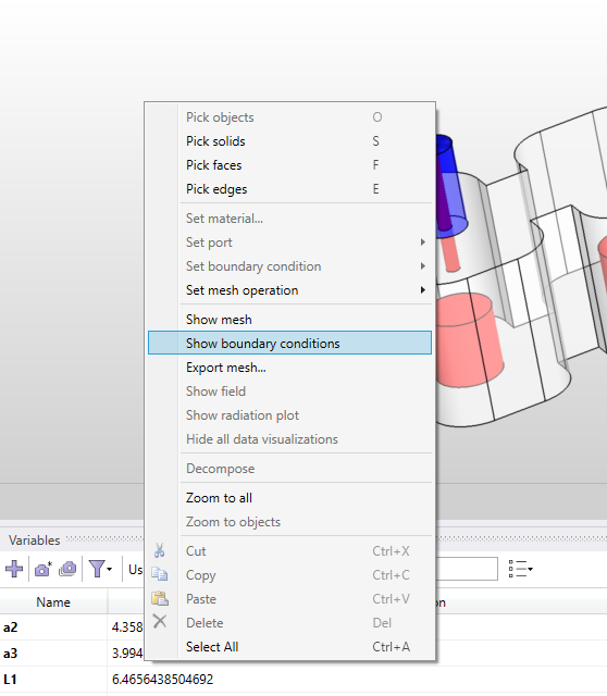
When working with complex structures where many boundary conditions are set, it is often hard to confirm whether the resulting simulation domain is set correctly. A convenient tool for checking boundary conditions is boundary conditions visualization which displays boundary condition types in the Scene view. When the view is enabled each face of structure is assigned a color based on boundary condition type allowing them to be easily distinguished from each other. The colors are described in a legend displayed in the top left corner of the Scene. To add a boundary conditions visualization select "Show boundary conditions" from the Scene context menu (Fig.4.4).

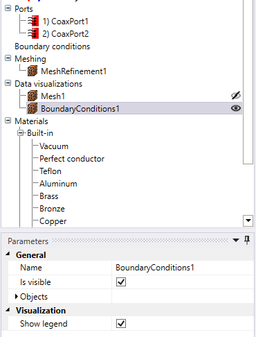
Once added the visualization will be visible in the project tree (Fig.4.5). Boundary visualization parameters are:

• • Name: the name of the visualization.

• • Is visible: indicates whether visualization is displayed or not.

• • Objects: not used.

• • Show legend: indicates whether visualization legend is displayed or not.

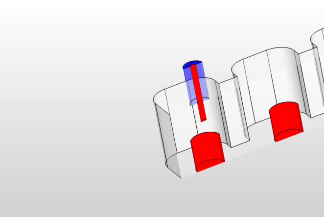
Boundary conditions view displays faces in opaque colors which means most of structure is obstructed from the view. In order to view entire structure cut view can be enabled as described in Section 3.1.1.