3 Geometry modeler
InventSim has the capability to construct computer models of two-dimensional and three-dimensional geometrical structures. The main part of the application is the modeler: a 3D editor that allows you to create and modify geometrical models of 3D and 2D structures.
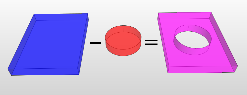
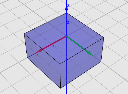
The modeling is based on the Constructive Solid Geometry (CSG) technique. Complex geometries can be created from simple objects, known as primitives, and then modified and/or subjected to Boolean operations. For example, creating a box with a cylindrical hole in the center is achieved by creating a box first, then creating a cylinder and subtracting it from the box, as seen in the picture 3.1
All operations on structures are parameterized: after the operations have been performed, their parameters can still be changed. For example, after creating a box, its position and dimensions can be changed without having to remove and create the box again. The operations performed on a structure form a list. It is executed from top to bottom in order to create the final structure. List of the operations can be seen as a blueprint for the structure. For example, this is the operation list of the structure seen above:
-
• Create a box.
-
• Create a cylinder in the center of the box.
-
• Subtract the cylinder from the box.
When the list is executed in that particular order, the result is a box with a hole inside it. As mentioned above, each operation is parameterized, so that position and dimensions of the box (as well as those of the cylinder) can later be changed without requiring you to recreate the entire structure. Each time you change the operation parameter, the structures rebuild themselves according to the new specification.
The modeler requires a coordinate system because it works in 3D space. It exclusively uses Cartesian right-handed coordinate systems. The default system is the global coordinate system, which cannot be deleted or modified. Other systems, which are related to the global system (or another, previously defined system), can be added. One of the coordinate systems is always active, which means that newly added operations will use that system as a reference. Each operation can have a different coordinate system assigned. Coordinate systems are parameterized in the same way as operations: changing one of the parameters causes the structure to be rebuild.
3.1 Controlling 3D view
You can move (pan), rotate and zoom the camera using the mouse, while pressing the necessary key. Normally, the middle mouse button (MMB) and mouse scroll are used to manipulate the camera, but if these are not available, you can use the right mouse button (RMB) as well. The table 1 explains how to manipulate the camera in both cases.
| Action |
With scroll/middle mouse button |
Without scroll/middle mouse button |
| Move |
Hold Ctrl and MMB while moving the mouse |
Hold Ctrl and RMB while moving the mouse |
| Rotate |
Hold MMB while moving the mouse |
Hold Ctrl+Shift and RMB while moving the mouse |
| Zoom |
Use the mouse scroll |
Hold Shift while moving the mouse |
By default, the camera rotates around the center point, which is the center for all objects, and with the Z-axis as its rotation axis. This allows you to rotate the camera around the entire scene. Alternative camera rotation mode can be enabled by moving the mouse cursor close to the left (or right) edge of the 3D View (the mouse cursor should change to "two arrows" cursor) and then rotating the view in the same way as described above. In this mode, the camera can be rotated around its own axis.
Furthermore, camera can be automatically positioned so that all structures are seen by using "Zoom to all commands" from the context menu. Similarly, the camera can be zoomed to a particular object(s) by first selecting the desired object and then clicking "Zoom to objects" from the context menu.
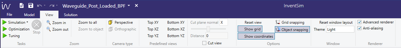
Perspective and Orthographic camera projections can be changed by selecting the appropriate button from the toolbar, as seen in Fig. 3.2.
3.1.1 Cut view
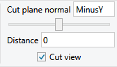
Cut view allows to render only part of the scene to better visualize some aspects of the project, for example to view internal parts of opaque objects. In order to view entire structure cut view can be enabled from the View ribbon menu by clicking on "Cut view" checkbox as shown in Fig.3.3. When enabled only part of the scene is rendered i.e. a part defined by the cut of 3D scene by a specified plane. The plane is defined by the plane normal and a distance which can be set in "Cut view" section of "View" ribbon (Fig.3.3).
3.2 Coordinate systems
The modeler uses coordinate systems to specify positions, define planes and directions in three-dimensional space. It exclusively uses Cartesian right-handed coordinate systems. The default system, named the global system cannot be modified or deleted and it is used internally by the geometry kernel. Other systems which are related to the global system (or another, previously defined system) can be added.
3.2.1 Planes
Some tools and operations require definition of the plane as a parameter value. Planes are associated with the active coordinate system which implicitly defines three planes:
-
• XY plane - the plane spanned by X and Y axes,
-
• XZ plane - the plane spanned by X and Z axes,
-
• YZ plane - the plane spanned by Y and Z axes.
Tools will use the active plane as the specified plane. Each of the planes can be chosen as the active plane by using the corresponding button from the toolbar, Fig. 3.4.

3.2.2 Directions
Some tools and operations require definition of the direction, for example rotation of objects requires definition of the axis of rotation. The direction used by the tool is the axis perpendicular to the active plane:
-
• for XY plane - Z-axis,
-
• for XZ plane - Y-axis,
-
• for YZ plane - X-axis.
3.2.3 Operations on coordinate systems
Adding
To add a coordinate system, select "Add command" from the toolbar. Specify the origin of the coordinate system by selecting the position with the mouse and clicking LMB or typing it after pressing Tab. The new coordinate system
will be relative to the previously active coordinate system. Once the system is added, its properties (like origin or rotation angles) can be modified in the parameters tab.
Moving
To move a coordinate system, i.e. change its origin, select it first and then select "Move" from the toolbar. Next, specify the new origin by selecting the position with the mouse and clicking LMB or typing it after pressing Tab.
Alternatively, enter the new origin in the parameters tab.
Rotating
To rotate a coordinate system, select the system in the project tree. Then, select the axis of rotation by selecting the correct active plane. Select "Rotate" from the toolbar. Now you can specify the angle by moving the mouse and
clicking LMB or typing it after pressing Tab. Alternatively, enter the new angle in the parameters tab.
Deleting To delete a coordinate system, select it in the project tree and then select "Delete" from the context menu. Coordinate systems used by an object cannot be deleted. In such a case, an error message will be shown.
3.3 Objects
The main part of the application is the modeler, a 3D editor allowing you to create and modify geometrical models of 3D and 2D structures. The modeler has the capability to model one, two and three-dimensional geometrical structures in 3D space.
The modeling is based on the Constructive Solid Geometry (CSG) technique. Complex geometries can be created from simple objects, known as primitives, and then modified and/or subjected to Boolean operations. For example, creating a box with a cylindrical hole in the center is achieved by creating a box first, then creating a cylinder and subtracting it from the box, as seen in the picture below.
All operations on structures are parameterized: after the operations have been performed, their parameters can still be changed. For example, after creating a box, its position and dimensions can be changed without having to remove and create the box again. The operations performed on a structure form a list, which is executed from top to bottom in order to create the final structure. List of operations can be seen as a blueprint for the structures. For example, this is the operations list of the structure seen above: Create a box. Create a cylinder in the center of the box. Subtract the cylinder from the box. When it is executed in that particular order, it results with a box with a hole in it. As mentioned above, each operation is parameterized, so that the position and dimensions of the box (as well as those of the cylinder) can later be changed without requiring you to recreate the entire structure. Each time you change the operation parameter, the structures rebuild themselves according to the new specification.
The purpose of the modeler is to model geometrical structures. Structures are divided into logical entities called SimObjects: one is made of structures of the same category (only solids, only faces or only one-dimensional objects) that share some of properties. For example all solids in a SimObject are assumed to be made of the same material.
3.3.1 Primitives
The building blocks of every modeled object are primitives, grouped in three categories. The first one is the three-dimensional closed solids, for which the available primitives are:
-
• Box
-
• Cylinder
-
• Cone
-
• Sphere
-
• Torus
The other category is the two-dimensional flat faces, and the list of primitives is as follows:
-
• Rectangle
-
• Circle
-
• Ellipse
-
• Polygon
Finally, the last group are 1D objects:
-
• Line
-
• Polyline
-
• B-spline
-
• Arc of circle
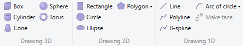
Each primitive can be constructed by selecting an appropriate tool from the toolbar (Fig.3.5. For example, creating a box requires the "Box" tool from the "Drawing 3D" toolbar section. The tools are interactive and the parameters of a particular object are set using either the mouse or pressing Tab and typing the exact values.
New objects are added with the "Create" operation located at the top of operations list. These operations are responsible for constructing objects and defining their geometrical parameters, i.e. its origin (common parameter P0) or its dimensions.
When selecting a drawing tool, the active coordinate system as well as the active plane of that system are used as appropriate parameter values of the "Create" operation.
To properly model 2D objects, InventSim requires them to be drawn on the surfaces or walls associated to 3D objects!
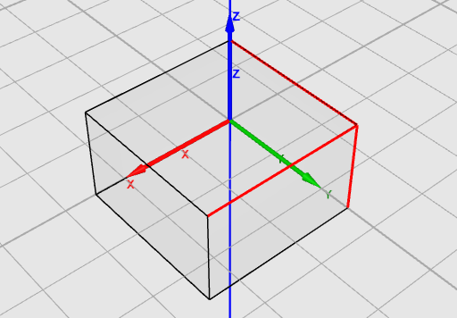
3.3.2 Box
A box is defined as a cuboid with its faces parallel to the coordinate system axes. To add a box, select the "Box" tool, specify its origin and then specify its X, Y and Z dimensions (Fig.3.6).
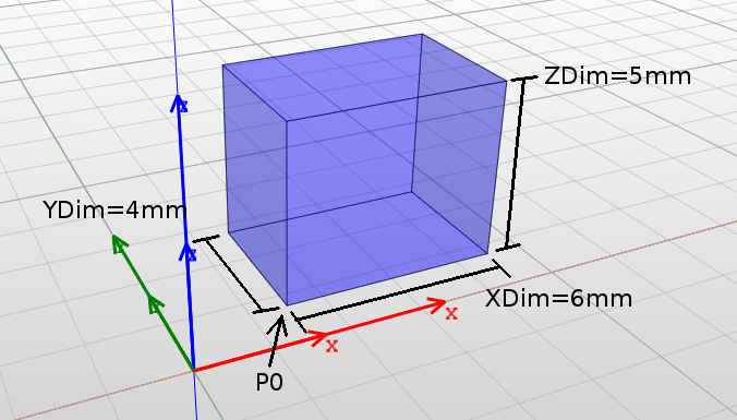
Boxes are constructed by CreateBox operation and the parameters are:
-
• Coordinate System: Assigned coordinate system.
-
• Plane: Irrelevant for the box.
-
• P0: Origin of the box: the position of one of its corners.
-
• XDim: Width of the box in X-axis.
-
• YDim: Width of the box in Y-axis.
-
• ZDim: Width of the box in Z-axis.
Remarks:
-
• Faces are parallel to the coordinate system axes and cannot be skewed.
-
• Width values can be negative. In such a case the box will be created as if the corresponding axis had the opposite direction.
-
• Faces name correspond to coordinate system planes: BottomXY and TopXY for faces parallel to XY plane, BottomXZ and TopXZ parallel to XZ plane, BottomYZ and TopYZ parallel to YZ plane.
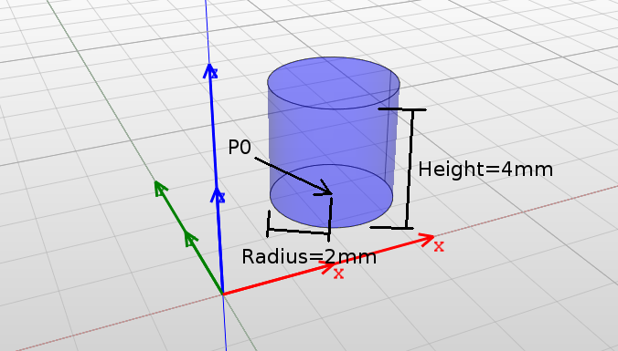
3.3.3 Cylinder
A cylinder is defined as a solid that has two parallel, circular bases connected by a curved surface. The orientation of the cylinder, i.e. its axis, is set as the direction perpendicular to the active plane of the active coordinate system. To add a cylinder, select the "Cylinder" tool, specify its origin and then specify its radius and height (Fig.3.7).
Cylinders are constructed by CreateCylinder operation and the parameters are:
-
• Coordinate System: Assigned coordinate system.
-
• Plane: Defines the axis of the cylinder, which is a vector normal to the active system plane.
-
• P0: Origin of the cylinder: the center of its bottom base.
-
• Radius: Radius of the cylinder.
-
• Height: Height of the cylinder: its length along the axis.
Remarks:
-
• The axis of the cylinder is perpendicular to the plane of the coordinate system and cannot be changed.
-
• Height can be negative. In such a case the cylinder will be created as if the axis had the opposite direction.
-
• Radius must not be negative.
-
• Face name are: BottomBase and TopBase for cylinder bases and Side for cylindrical face.
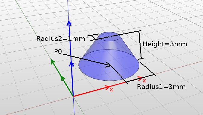
3.3.4 Cone
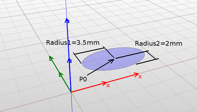
A cone is defined as a solid that tapers smoothly from a flat, circular base to a point or another base (truncated cone). The axis of the cone is perpendicular to the base and is set as the direction perpendicular to the active plane of the active coordinate system. To add a cone, select the "Cylinder" tool, specify its origin and then specify the radii of the bottom and the base (Fig.3.8).
Cones are constructed by CreateCone operation and the parameters are:
-
• Coordinate System: Assigned coordinate system.
-
• Plane: Defines the axis of the cone, which is a vector normal to the system active plane.
-
• P0: Origin of the cone: the center of its bottom base.
-
• Radius1: Radius of the bottom base.
-
• Radius2: Radius of the top base.
-
• Height: Height of the cone: its length along the axis.
Remarks:
-
• The axis of the cone is perpendicular to the plane of the coordinate system and cannot be changed.
-
• Height can be negative. In such a case the cone will be created as if the axis had the opposite direction.
-
• Neither Radius1 nor Radius2 can be negative.
-
• Face name are: BottomBase and TopBase for cone bases and Side for conical face.
3.3.5 Sphere
A sphere is defined as a solid with one face, which is a set of all points that are located at a certain distance (radius) from a point (origin). To add a sphere, select the "Sphere" tool and specify its origin and radius (Fig.3.9).
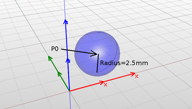
The spheres are constructed by CreateSphere operation and the parameters are:
-
• Coordinate System: Assigned coordinate system.
-
• Plane: Irrelevant for the sphere.
-
• P0: Origin of the sphere: its center.
-
• Radius: Radius of the sphere.
Remarks:
-
• Radius must not be negative.
-
• Face name is SphereFace.
3.3.6 Torus
A torus is defined as a solid with one face, which is created as a surface of revolution by revolving a circle around an axis. The axis is perpendicular to the active plane of the active coordinate system and the center of revolution is the torus origin point. To add a torus, select the "Torus" tool and specify its origin and both radii.
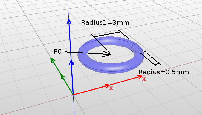
Toruses are constructed by CreateTorus operation and the parameters are:
-
• Coordinate System: Assigned coordinate system.
-
• Plane: Defines axis of the torus which is a vector normal to the system active plane.
-
• P0: Origin of the torus: its center.
-
• Radius1: Radius of the torus: distance from the origin to the center of revolving circle.
-
• Radius2: Radius of the toroidal face.
Remarks:
-
• Neither Radius1 nor Radius2 can be negative.
-
• Face name is Torus.
3.3.7 Helix
A helix is defined as a solid with one face, which is created as a surface of revolution by revolving a circle around an axis. The axis is perpendicular to the active plane of the active coordinate system and the center of revolution is the torus origin point. To add a torus, select the "Torus" tool and specify its origin and both radii.
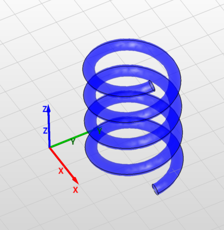
Helices are constructed by CreateHelix operation and the parameters are:
-
• Coordinate System: Assigned coordinate system.
-
• Plane: Defines axis of the helix which is a vector normal to the system active plane.
-
• P0: Origin of the helix, the point on bottom end of the helix axis.
-
• Radius1: Radius of the bottom end.
-
• Radius2: Radius of the top end.
-
• Turns: Number of helix turns.
-
• Angle: Helix angle.
-
• Profile radius: Radius of the helix profile.
-
• Twist: Helix twist direction.
Remarks:
-
• Neither Radius1 nor Radius2 can be negative.
-
• Faces names are: HelixFace0 and HelixFace2 for bottom and top faces respectively, HelixFace1 for the side face.
3.3.8 Rectangle
A rectangle is defined as a two-dimensional face with two pairs of edges and four right angles. The face lies on an active plane of the active coordinate system (XY, XZ or YZ). To add a rectangle, select the "Rectangle" tool, specify its origin and then specify width and height (Fig.3.12).
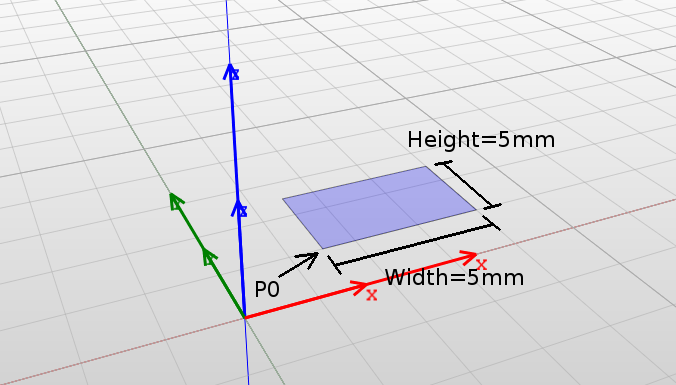
Rectangles are constructed by CreateRectangle operation and the parameters are:
-
• Coordinate System: Assigned coordinate system.
-
• Plane: Defines the plane on which the face lies.
-
• P0: Origin of the rectangle: position of one of its corners.
-
• Width: Length of the rectangle in the first dimension.
-
• Height: Length of the rectangle in the second dimension.
Remarks:
-
• Width and Height are defined as lengths in the first and the second dimensions of the plane. For example, if the XZ plane is set, Width is the length in X dimension and Height is the length in Z dimension.
-
• Width and Height can be negative. In such a case the rectangle will be created as if the axis had the opposite direction.
-
• 2D objects are always created on XY, XZ or YZ planes and can later be moved to other locations using the "Move" operation.
-
• Face name is Rectangle.
3.3.9 Circle
A circle is defined as a two-dimensional face bounded by one, circular edge. The face lies on a plane parallel to the active plane of the active coordinate system. To add a circle, select the "Circle" tool and specify its origin and radius (Fig.3.13).
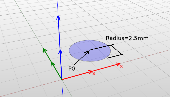
Circles are constructed by CreateCircle operation and the parameters are:
-
• Coordinate System: Assigned coordinate system.
-
• Plane: Defines the plane on which the face lies.
-
• P0: Origin of the circle: its center.
-
• Width: Length of the circle in the first dimension.
-
• Height: Length of the circle in the second dimension.
Remarks:
-
• Radius must not be negative.
-
• Face name is Circle.
3.3.10 Ellipse
An ellipse is defined as a two-dimensional face bounded by an ellipse edge. The face lies on a plane parallel to the active plane of the active coordinate system. To add an ellipse, select the "Ellipse" tool and specify its origin and both radii (Fig.3.14).
Ellipses are constructed by CreateEllipse operation and the parameters are:
-
• Coordinate System: Assigned coordinate system.
-
• Plane: Defines the plane on which the face lies.
-
• P0: Origin of the ellipse: its center.
-
• Width: Length of the ellipse in the first dimension.
-
• Height: Length of the ellipse in the second dimension.
Remarks:
-
• Radius1 and Radius2 are defined as length in the first and the second dimensions of the plane. For example, if the XZ plane is set, Radius1 is the length in X dimension and Radius2 is the length in Z dimension.
-
• Radius1 and Radius2 must not be negative.
-
• Face name is Ellipse.
3.3.11 Polygon
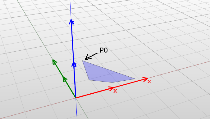
A polygon is defined as a two-dimensional face bounded by a set of straight edges. Only simple polygons are allowed i.e. polygons that do not intersect themselves and have no hole. The face lies on a plane parallel to the active plane of the active coordinate system.
To add a polygon, select the "Polygon" tool and specify its origin as well as the remaining polygon vertexes: press Shift+Enter to finish adding vertexes (Fig.3.15).
Additionally regular polygons can be created by specifying the origin, one of the vertices and the number of sides.
Polygons are constructed by CreatePolygon operation and the parameters are:
-
• Coordinate System: Assigned coordinate system.
-
• Plane: Defines the plane on which the face lies.
-
• P0: Origin of the polygon: position of one of its corners.
-
• Number of points: Number of vertexes (read-only).
-
• Points: List of the positions of vertexes.
Remarks:
-
• List of vertex positions cannot be changed, only the position values can be.
-
• Face name is either RegularPolygon or Polygon.
3.3.12 Line
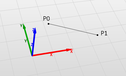
A line is a straight line segment connecting two points. The line lies on a plane parallel to the active plane of the active coordinate system.
To add a line, select the "Line" tool and specify its two points (Fig.3.16).
Lines are constructed by CreateLine operation and the parameters are:
-
• Coordinate System: Assigned coordinate system.
-
• Plane: Defines the plane on which the line lies.
-
• P0: start point.
-
• P1: end point.
Remarks:
-
• Edge name is Line.
3.3.13 Polyline
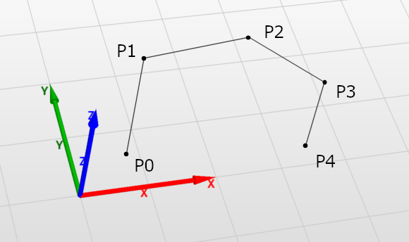
Polylines are sets of connected straight line segments connecting defined points. Polylines lie on a plane parallel to the active plane of the active coordinate system.
To add a polyline, select the "Polyline" tool and specify its points (Fig.3.17).
Polylines are constructed by CreatePolyline operation and the parameters are:
-
• Coordinate System: Assigned coordinate system.
-
• Plane: Defines the plane on which the line lies.
-
• Number of points: cannot be changed after polyline is created.
-
• Points: collection of points which are connected by lines.
Remarks:
-
• Edge names are PolyLine_PartN where N is the index of the edge (starting with 0).
3.3.14 B-spline
In InventSim B-spline is a collection of piecewise polynomial curves passing through an array of points. It lies on a plane parallel to the active plane of the active coordinate system.
To add a B-spline, select the "B-spline" tool and specify its points (Fig.3.18).
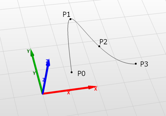
B-splines are constructed by CreateBSpline operation and the parameters are:
-
• Coordinate System: Assigned coordinate system.
-
• Plane: Defines the plane on which the edge lies.
-
• Number of points: cannot be changed after B-spline is created.
-
• Points: collection of points which are connected by splines.
-
• Is periodic: if set BSpline curve will be periodic and closed. In this case, the junction point is the first point of the Points.
Remarks:
-
• There must be at least two points.
-
• Edge name is "BSpline".
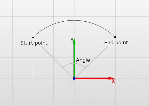
3.3.15 Arc of circle
InventSim allows to create sections of circle in several ways depending on what parameters are more convenient for the user. The options are:
-
• Center, radius and angles
-
• Center, start and end
-
• Three points
-
• Start, end and radius
-
• Start, end and angle - makes an arc of circle from two points i.e. starting and end point and an angle formed by lines connecting the circle center and the two points.
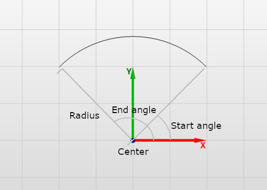
Makes an arc of circle from a circle (defined by its center and radius) and two angles. The arc spans between two points: start point and end point. Both points are calculated based on center of the circle and angles formed by the primary axis of the coordinate system and the lines connecting the starting point and the end point with the center.
To add a arc of circle, select the "Arc of circle" tool, then "Center, radius and angles" tool mode.
The arc is constructed by CreateArcOfCircle operation and the parameters are:
-
• Coordinate System: Assigned coordinate system.
-
• Plane: Defines the plane on which the curve lies.
-
• Definition: cannot be changed after arc of circle is created.
-
• Center point: center of the circle.
-
• Radius: radius of the circle.
-
• Start angle: angle between first plane axis and line connecting circle center with start point of the arc.
-
• End angle: angle between first plane axis and line connecting circle center with end point of the arc.
Remarks:
-
• Radius must be positive.
-
• Curve name is "ArcOfCircle".
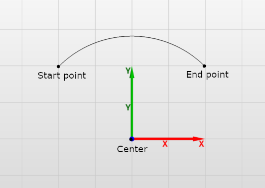
Makes an arc of circle from a circle (defined by its radius) and two points being start and end point.
To add a arc of circle, select the "Arc of circle" tool, then "Center, start and end" tool mode.
The arc is constructed by CreateArcOfCircle operation and the parameters are:
-
• Coordinate System: Assigned coordinate system.
-
• Plane: Defines the plane on which the curve lies.
-
• Definition: cannot be changed after arc of circle is created.
-
• Center point: center of the circle.
-
• Start point: start point of the arc.
-
• End point: end point of the arc.
Remarks:
-
• Curve name is "ArcOfCircle".
Make an arc of circle which spans between two points and having circle radius calculated based on a third point located on the arc between the first two points.
To add a arc of circle, select the "Arc of circle" tool, then "Center, radius and angles" tool mode.

The arc is constructed by CreateArcOfCircle operation and the parameters are:
-
• Coordinate System: Assigned coordinate system.
-
• Plane: Defines the plane on which the curve lies.
-
• Definition: cannot be changed after arc of circle is created.
-
• Start point: start point of the arc.
-
• End point: end point of the arc.
-
• Arc point: point located on the arc between start and end points.
Remarks:
-
• Curve name is "ArcOfCircle".
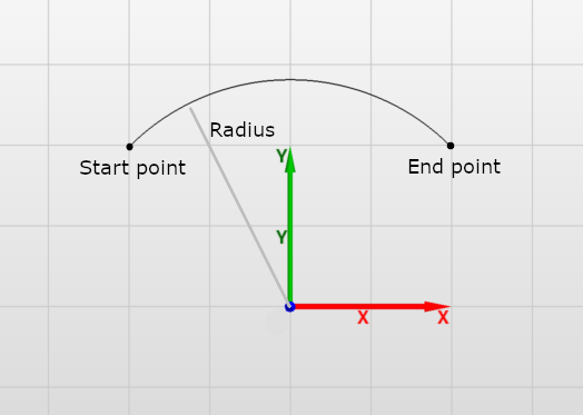
Makes an arc of circle from two points i.e. start and end point and the circle radius.
To add a arc of circle, select the "Arc of circle" tool, then Start, end and radius" tool mode.
The arc is constructed by CreateArcOfCircle operation and the parameters are:
-
• Coordinate System: Assigned coordinate system.
-
• Plane: Defines the plane on which the curve lies.
-
• Definition: cannot be changed after arc of circle is created.
-
• Start point: start point of the arc.
-
• End point: end point of the arc.
-
• Radius: radius of the circle.
-
• Positive angle:
Remarks:
-
• Curve name is "ArcOfCircle".
Makes an arc of circle from two points i.e. start and end point and an angle between lines connecting start and end points with the circle center.
To add a arc of circle, select the "Arc of circle" tool, then "Start, end and angle" tool mode.
The arc is constructed by CreateArcOfCircle operation and the parameters are:
-
• Coordinate System: Assigned coordinate system.
-
• Plane: Defines the plane on which the curve lies.
-
• Definition: cannot be changed after arc of circle is created.
-
• Start point: start point of the arc.
-
• End point: end point of the arc.
-
• Angle: angle between lines connecting start and end points with the circle center.
Remarks:
-
• Curve name is "ArcOfCircle".
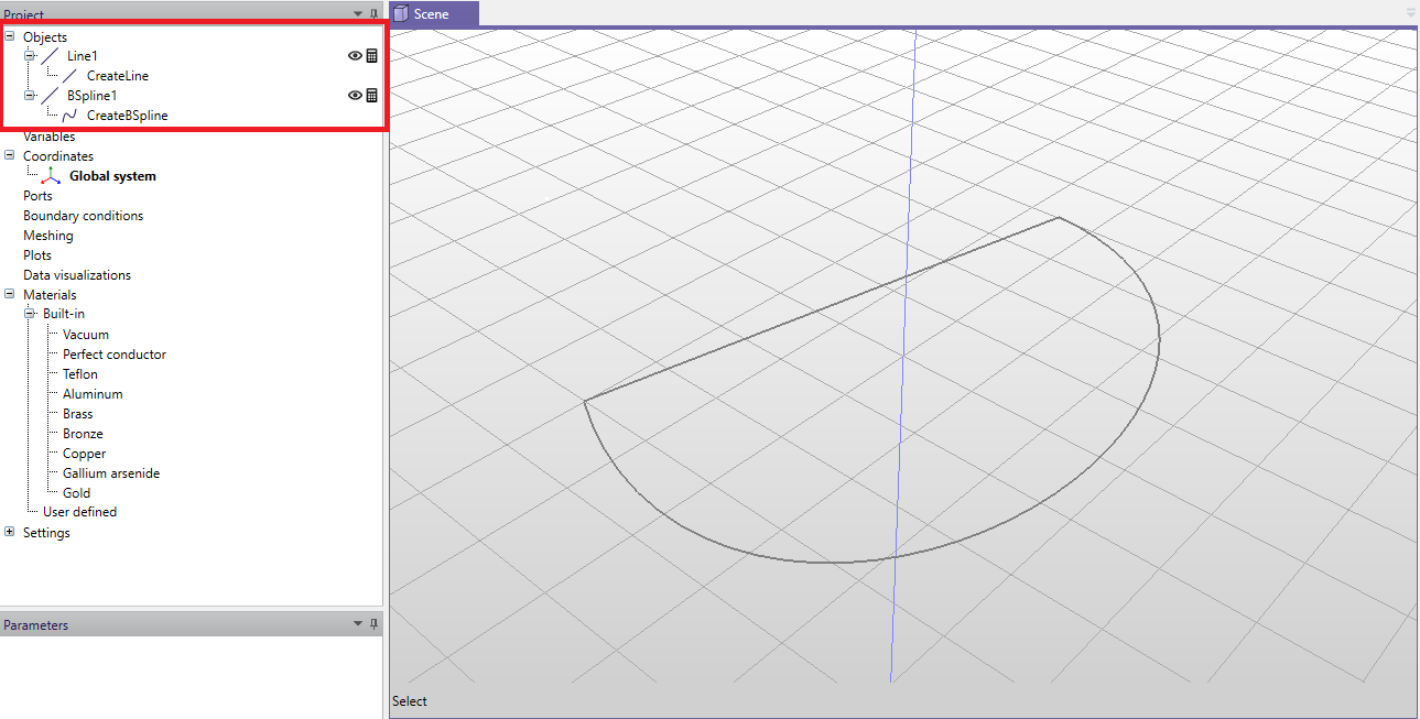
3.3.16 Face from closed contour
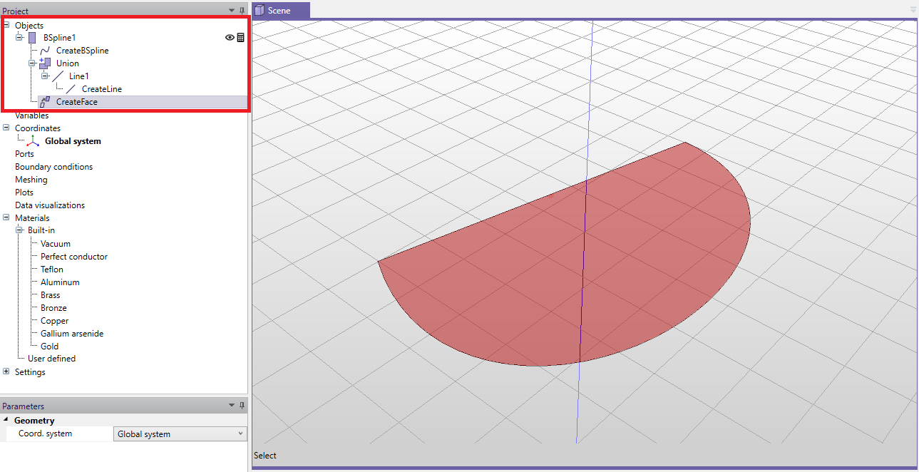
When the user draws a closed contour using 1D drawing tools, it is possible to transform it to 2D face. To use this feature, draw a contour that can consist of several 1D objects, as shown in Fig. 3.24. Then, unite the 1D objects into one closed contour, select it and click icon make face (
![]() ). The result of this operation is a 2D face, as shown in Fig. 3.25.
). The result of this operation is a 2D face, as shown in Fig. 3.25.
3.4 Boolean operations
To create geometry models that are more complex than the simple primitives, Boolean operations should be used. Boolean operations available in the modeler are an extrapolation of Boolean algebra of sets.
Notice: When using Boolean operations on the objects, all arguments of Boolean operations are deleted - only the the resulting object of the operation is stored. In order to keep the copies of those argument objects please hold "Shift" when clicking the operation icon.
3.4.1 Union
This tool creates a union of two or more objects - i.e. it merges two or more objects together. If the two objects are disjoint, the result will be an object with two separate parts. The operation can be described by the following equation:
\begin{equation} A_R = A_1 + A_2 + ... + A_n \end{equation}
where \(A_R\) is the operation result and \(A_i\), (\(i=1,2,\ldots , n\)) are the operation arguments.
In order to unite two or more objects, select them, then select the "Unite" tool from the toolbar. The order in which objects are selected is not relevant.
3.4.2 Subtraction
This tool creates a difference of two or more objects - i.e. it subtracts one or more objects from a single object. The operation can be described by the following equation:
\begin{equation} A_R = A_1 - A_2 - ... - A_n \end{equation}
where \(A_R\) is the operation result and \(A_i\), (\(i=1,2,\ldots , n\)) are the operation arguments.
In order to subtract two or more objects from a desired object, select it first. Then select the object(s) you wish to subtract. After that, select the "Subtract" tool from the toolbar. The order of your selection is important. The object from which you want to subtract must be selected first. Then the rest of objects can be selected.
3.4.3 Intersection
This tool creates an intersection of two or more objects - i.e. it creates an object(s) which consists of the common part of the selected objects. The operation can be described by the following equation:
\begin{equation} A_R = A_1 \times A_2 \times ... \times A_n \end{equation}
where \(A_R\) is the operation result and \(A_i\), (\(i=1,2,\ldots , n\)) are the operation arguments.
In order to intersect two or more objects, select them, then select the "Unite" tool from the toolbar. The order in which the objects are selected is not relevant.
3.5 Modifications
Thanks to parametrization of objects, structures can be modified after their construction by changing the values of their parameters. Nevertheless, a set of modification tools is available for additional modifications. Using the tools requires selecting the object which will be the subject of the modification. After specifying the modification parameters values, an appropriate operation will be added to the objects operations list.
3.5.1 Move
This tool moves the object by a specified offset, defined as a three-dimensional vector. To move an object, select it first and then select the "Move" tool from the toolbar. To move the object, specify the starting point and the final point of the movement.
Moving object is performed by the "Move" operation which has the following parameters:
-
• Coordinate System: Assigned coordinate system.
-
• Offset: Offset by which the object is moved.
3.5.2 Rotate
This tool rotates the object by a specified angle around an axis. The axis is determined by the active coordinate system and the active plane upon selecting the tool. It is set as the direction perpendicular to the active plane with the center of rotation being the origin of the active coordinate system. For example, if the YZ plane is the active plane, the axis will be a vector parallel to X-axis. To rotate the object, select it first and then select the "Rotate" tool from the toolbar. Specify the angle of rotation either by moving the mouse and clicking LMB or by typing the exact value after pressing Tab.
Rotation of objects is performed by the "Rotate" operation which has the following parameters:
-
• Coordinate System: Assigned coordinate system.
-
• Plane: Determines the axis of rotation.
-
• Angle: Angle of rotation.
3.5.3 Reflect
This tool reflects an object across a specified plane. To reflect an object, select it first and then select the "Reflect" tool from the toolbar. Specify the plane of rotation by moving the mouse over 3D View and click LMB.
Reflecting object is performed by the "Reflect" operation which has the following parameters:
-
• Coordinate system: Assigned coordinate system.
-
• Plane: Plane by which the object is reflected.
3.5.4 Clone along line
This tool takes an object and creates one (or more) exact copy of it. The cloned objects are placed along a specified line, each displaced by a specified distance. Construction of the clones is done by the CreateByCloning operation which is added to the top of the clones operations list. Any changes to the original object operations parameters prior to cloning will result in reconstruction of the clones.
To clone an object along a line, select it and then select "Clone along line tool" from the toolbar. Determine the displacement of the clones by specifying the starting and the final points and then enter the wanted number of clones.
Cloning along line is performed by "CloneAlongLine" operation which has the following parameters:
-
• Coordinate System: Assigned coordinate system.
-
• Copies: Number of created clones.
-
• Offset: Offset by which each of the clones is displaced.
Remarks:
-
• Clones are completely independent - i.e. modifying or deleting one of the clones will not affect the rest of the clones, nor the original object.
-
• Deleting the original object does not affect the clones.
-
• Deleting CloneAlongLine operation from the original object operations list removes all the clones.
3.5.5 Clone around axis
This tool takes an object and creates one (or more) exact copy of it. The clones are placed around a specified point, each rotated by a specified angle. The axis is determined by the active coordinate system and the active plane upon selecting the tool. It is set as the direction perpendicular to the active plane with the center of rotation being the origin of the active coordinate system. Construction of the clones is done by CreateByCloning operation which is added to the top of the clones operations list. Any changes to original object operations parameters prior to cloning results in reconstruction of the clones.
To clone an object around axis, select it first and then select "Clone around axis" tool from the toolbar. Specify the angle of rotation either by moving the mouse and clicking LMB or by typing the exact value after pressing Tab key and then entering the number of clones.
Cloning around axis is performed by "CloneAroundAxis" operation which has the following parameters:
-
• Coordinate System: Assigned coordinate system.
-
• Copies: Number of created clones.
-
• Plane: Determines the axis of rotation.
-
• Angle: Angle by which each of the clones is rotated.
Remarks:
-
• Clones are completely independent - i.e. modifying or deleting one of the clones will not affect the rest of the clones nor the original object.
-
• Deleting the original object does not affect the clones.
-
• Deleting CloneAroundAxis operation from the original object operations list removes all the clones.
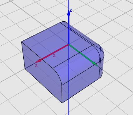
3.5.6 Fillet edge
This tool creates fillets which are the rounding of the edges of solids. To use the tool, select "Pick edges" and then select one or more edges. Use the toolbar and select "Fillet edge". You will be asked for the radius of the fillet (Fig.3.26).
Remarks:
-
• If the fillet cannot be created or fails to generate, the result will be equivalent to Radius=0.
-
• Creating fillets on some edges will result in having fillets on other edges.
3.5.7 Edge chamfering
This modification is similar to edge filleting, but the edges are cut as opposed to being rounded. (Fig.3.27).
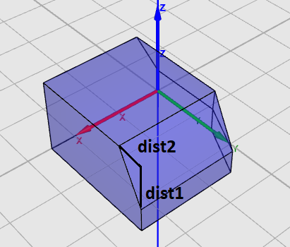
Edge chamfering is performed by "ChamferEdge" operation which has the following parameters:
-
• Coordinate System: Assigned coordinate system.
-
• Dist1: Distance from one edge to be cut.
-
• Dist2: Distance from the other edge to be cut
3.5.8 Extrude
Extruding is an operation that modifies the 2D object into a solid. Three variants of extrusion are available in InventSim:
-
• Extrude along normal: It is the simplest variant, where the 2D object is extruded along a vector normal to its surface. For example, extrusion of a rectangle would give you a box.
-
• Extrude along vector: In this case the extrusion is made along an arbitrary, used-defined vector.
-
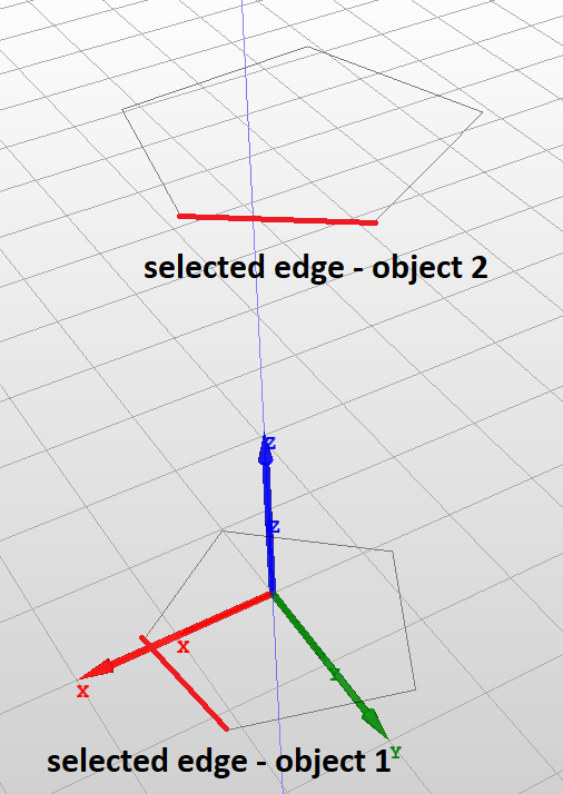
• Extrude ruled: With this operation, is is possible to construct a solid with a ruled surface. To do so, the user needs to provide two 2D objects with the same number of edges and then select one edge in each object (Fig. 3.28). The operation would connect the nodes of the objects with straight lines.
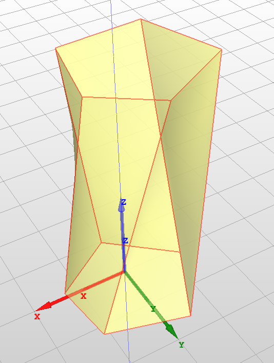
3.5.9 Revolution around axis
The revolution operation transforms a 2D object into a 3D solid by rotating the surface around an axis of rotation.
The "Revolution" operation has the following parameters:
-
• Coordinate System: Assigned coordinate system.
-
• Plane: Plane of rotation
-
• Angle: Angle of rotation
Remarks:
-
• 2D object can not lay down on the plane of rotation.
3.6 Selecting objects
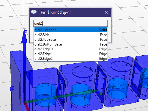
To access the object properties, modify object faces or edges, you need to select proper object, its face or edge. This can be done using the mouse, but also with the special dialog box "Find SimObject" accessible with "Ctrl+T" shortcut (Fig. 3.29).
3.7 Hiding and disabling calculation of objects
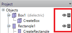
By using the icons on the object list in the project tree panel (Fig.3.30, you can easily control the properties of the object, such as:
-
• Visibility: select this icon (
 ) to enable/disable object display in the 3D view window.
-
• Activity: select this icon (
 ) to exclude the object from calculations (object is still visible in the 3D view, but is not taken into account during simulations).
3.8 Variables and equations
One of the basic features of InventSim is model parametrization by using variables. This feature is essential for efficient and successful design, since it allows you to change and control the model geometry in an easily accessible way. In principle, there are algebraic expressions which, when evaluated, represent floating point values. Variables may be used as values of most of the parameters - instead of numerical values. Whenever a variable value changes, objects that use that variable are reconstructed with the new parameters values.
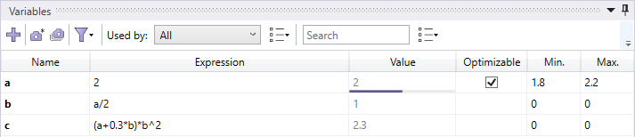
The variables are available in the variables panel, located by default below the scene view (Fig. 3.31). The panel presents all variables in a table form where each row shows parameters of a single variable. Above the table a toolbar is shown providing additional functionalities described below.
3.8.1 Adding variables
There are several ways to add a new variable:
-
• Right click on the "Variables" and select "New" from the context menu. A new variable will be added to the list of variables with the default name and the value of zero - the user can then modify the name and assign the value of the variable using the variable properties window.
-
• Click
 button in the toolbar.
-
• When creating/modifying an object and entering its dimensions you can input a string with the variable name and its value, for example entering the string "b=10.16" as the box size parameter "YDim"
-
• When creating/modifying an object and entering its dimensions you can input a string with the name of the variable. (for example "c") When no variable with that name is found, you will be asked about the value of that variable, as shown in Fig. 3.32.
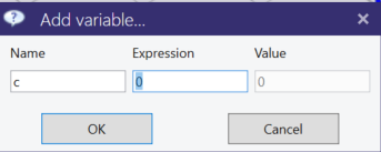
The variables can later be used in formulas (equations) that use the already defined variables. For example, if variables "a" and "b" exist within the project, we can enter an equation "c = a + b/2". Several mathematical functions can be used in the expression, like trigonometric functions \(sin(), cos()\) - a full list is shown in table 2. Predefined constants are shown in table 3.
3.8.2 Deleting variables
To delete a variable use one of the following actions:
-
• Select the variable from the list and press "Del" keyboard button.
-
• Select the varaible from the list and select "Delete" from the context menu.
Note that only unused variables can be deleted. An attempt to delete a referenced variable will result in an error.
3.8.3 Sorting and filtering
Variables list can be sorted by any of the parameters shown by clicking on a column header. By default the order in which variables are shown is the order in which they were added. Clicking one the column header sorts variables by that column in ascending order. Second click reverses sorting and the third resets sorting.
Additionally variables can be filtered in several ways to show:
-
• only optimizable variables
-
• only variables used in a particular object, coordinate system or material,
-
• only variables containing a specified text.
To show only optimizable variables click on
 button in the toolbar and check "Only optimizable" checkbox.
To display only variables used in the parameter values of a specific object, coordinate system, or material, select that object from the "Used by" drop-down list. Select "All" if you want to clear the filter. Additionally, a drop-down options menu is available where the user can specify the context in which variables are used. The "Include equations" option means that nested variables used in equations referenced in parameter values will also be shown. For example, if two variables are present, "a=1" and "b=a/2," and an object uses the variable "b," variable "a" will also be shown because it is used in the equation defining variable "b." The "Include coordinate systems" option allows including variables used in all coordinate systems referenced by the selected object.
To show only variables containing certain text, type that text in the "Search" text box. The options drop-down menu allows you to specify where the text will be searched: variable names and/or variable equations.
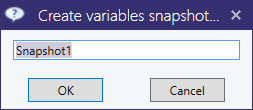
3.8.4 Variable snapshots
InventSim allows users to store sets of variable values for later use. These sets are called snapshots and contain all real valued variable values. To create and add a snapshot click on
 button in the toolbar. A dialog prompting for a snapshot name will appear (Fig.3.33). Click "OK" button to confirm the name and
add the snapshot. To view stored snapshots click on
button in the toolbar. A dialog prompting for a snapshot name will appear (Fig.3.33). Click "OK" button to confirm the name and
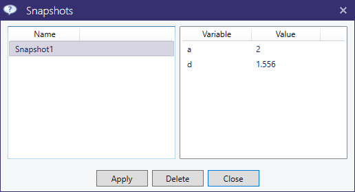
add the snapshot. To view stored snapshots click on
 button in the toolbar. Snapshots view will appear in a dialog window as shown in Fig.3.34. To delete a snapshot, select it in the left
pane and click on "Delete" button. To apply snapshot, select it in the left pane and click on "Apply" button.
button in the toolbar. Snapshots view will appear in a dialog window as shown in Fig.3.34. To delete a snapshot, select it in the left
pane and click on "Delete" button. To apply snapshot, select it in the left pane and click on "Apply" button.
3.8.5 Functions
| Symbol | Description |
| ̂ | Power |
| + | Add |
| - | Subtract |
| / | Divide |
| * | Multiply |
| cos() | Cosinus |
| sin() | Sinus |
| exp() | Exponential |
| ln() | Natural logarithm |
| tan() | Tangent |
| acos() | Arcus cosinus |
| asin() | Arcus sinus |
| atan() | Arcus tangent |
| sqrt() | Square root |
| cotan() | Cotangent |
| acotan() | Arcus cotangent |
| round(a, PRECISION) | Round number up to provided precision |
| ceil() | Smallest following integer |
| floor() | Largest previous integer |
| abs() | Module |
| log() | Common (base-10) logarithm |
| rad() | Convert degrees to radians |
3.9 CAD data exchange
InventSim supports the import and export operations of geometry models using the *.STEP file format (ISO 10303 - Standard for the Exchange of Product model data). With this feature, you can import complex geometry models from other CAD tools and export the geometry models for further processing. The import/export feature can be accessed using the toolbar icons shown in Fig.3.35. Compatibility issues: ] When importing complex geometries from a CAD package that uses other geometry processing kernels, please review the imparted model carefully, as models created with different CAD software are not always compatible with each other.
