8 Simulation options

Once the model is ready for simulation - i.e. the geometry, materials, boundary conditions, ports and mesh options are properly defined in the project, the last step before starting the simulation is to adjust the solution settings.

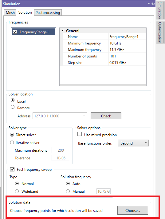
In InventSim, several settings for the solution phase are available in the "Solution" tab of the "Simulation" window hidden on the right part of the interface (Fig. 8.1). The settings include:

• • Setup of simulation frequencies.

• • Solver options.

• • Saving solution datasets.

8.1 Frequency plan

The purpose of the frequency sweep simulation is to obtain a structure response in the frequency domain by computing the response at defined frequency points.

Frequency points are defined in the "Frequencies" part of the "Solution" panel. Frequency points are specified in a form of frequency ranges, listed on left of the tab. A frequency range is defined as a set of points that is evenly distributed on the frequency axis, with the following parameters:

• • Name. The name of the frequency range.

• • Minimum frequency. The lower bound of the frequency range.

• • Maximum frequency. The upper bound of the frequency range.

• • Number of steps. The number of points in the frequency range.

• • Step size. The distance between the two closest frequency points in the frequency range.

To add a frequency range, select "Add" from the context menu of the left side of the tab. The new frequency range will be added with the default parameters and the default name.

To delete the frequency range, first select it in the list and then choose "Delete" from the context menu.

Frequency ranges can be made inactive in order to temporarily disable the simulation at some frequency points. Only the active frequency ranges are used during the frequency sweep simulation. To activate or deactivate a frequency range, select the checkbox on the left side of the frequency range name.

8.2 Solver options

The solver options are located just below the "Frequency plan" settings. The aim of those options is to give you better control of the solution phase. In general, every 3D FEM simulation of electromagnetic fields in the frequency domain involves a solution of a large, sparse linear system of equations in form:

\begin{equation} A \cdot x = b \end{equation}

where \(A\) is a sparse matrix, \(b\) is a block of right hand side vectors that correspond to excitations (modes) at ports, and \(x\) is a solution vector that represents the unknown fields inside of the structure. The equation is solved at every frequency point. The size of the linear system matrix \(A\), i.e. the number of the unknowns, depends on the model discretization and the order of the base function used to represent the fields.

8.2.1 Solver location

You can define the machine on which the solver process will run with this option. The default setting value is "Local" - i.e. the same machine on which the InventSim GUI application is running. The solver can be run, remotely, on another networked machine (with the necessary license) by selecting "Remote" and specifying the IP address and the port of the machine. After entering the machine parameters, use the "Check" button to check the remote solver response.

8.2.2 Solver type

This is the area in which InventSim allows you to setup the numerical techniques that will be used to solve a problem. These are the available options:

• • Direct solver. With the direct solver, the linear system of equations is solved by using sparse matrix factorization algorithms. In InventSim, we use Intel MKL Pardiso that has this option. In general, a direct solution of the problem is a memory consuming process, but as long as you have have enough memory to be able to factorize the matrix, this is the recommended setting. It is recommended to use this option if possible, especially when "Fast frequency sweep" is enabled.

• • Iterative solver. With this option, the solution phase is done with the iterative method (PCG) with the dedicated preconditioner. This setting is recommended for very large problems that cannot be solved with the "Direct" solver due to the "out of memory" problem. To use the iterative solver, you need to specify the maximum number of iterations that will be performed for each solution as well as the solution tolerance (defined as residual error of the solution). Please note that the convergence of a iterative solver cannot be guaranteed.

• • Mixed precision.In order to reduce the memory footprint during the solution phase, some stages of the solution can be performed using a single precision floating point number. Enabling this option will save some memory, but in rare cases it can lead to lower accuracy of the solution.

• • Base functions. With this option, you can specify the order of the base functions that will be used to represent the electromagnetic field.

  • – First order - the solver uses a linear vector functions defined over tetrahedron element (CTLN - constant tangential, linear normal).

  • – Second order - the solver uses a quadratic vector functions defined over tetrahedron element (LTQN - linear tangential, cubic normal).

  • – Third order - the solver uses a cubic vector functions defined over tetrahedron element (QTCuN - quadratic tangential, cubic normal).

  With the increase of the base function order, the problem size increases substantially. In practice we recommend using the default "Second order" option as it is a compromise between the accuracy of the solution and the solution time.

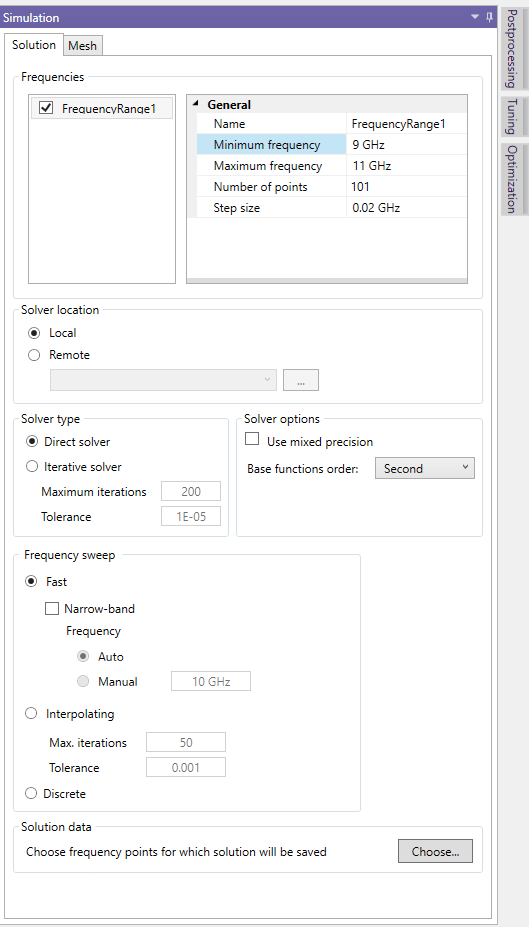
8.3 Frequency sweep type

With this option, you can choose between three different frequency sweep techniques: the ’Discrete Sweep’ the ’Fast Frequency Sweep’, and the ’Interpolating Sweep.’ The last two can expedite the evaluation of the transfer function at multiple frequency points.

The most general sweep is ’Discrete sweep.’ When selected, simulation is performed independently for every frequency point, which means that at each frequency point, a large linear problem has to be solved. If a substantial number of frequency points is defined in the frequency plan (tens or hundreds), this can lead to a long simulation time. At the same time, this option provides the most rigorous results. It is also recommended to use the discrete sweep when the number of points defined in the simulation is very low (i.e. below  10).

With the "Fast frequency sweep" enabled, the model of the transfer functions is constructed in an adaptive way: as the order of the model grows, the convergence of the transfer function is monitored. Usually, the numerical cost of creating such a model is much lower than a discrete sweep. In this mode, the wideband response in the frequency domain is extracted from the solution at a minimum number of frequency points - in some cases we can extract the wideband response even from a single frequency point! The efficiency of the fast frequency sweep depends on the number of resonances within the structure over the analyzed frequency band. If there are many resonances (tens/hundreds), the sweep may become less efficient, or could even fail. In this case, the direct sweep is recommended. Please note that the ’Fast Frequency Sweep’ cannot be used for simulation projects that involve dispersive materials like Debye dielectrics, ferrites, or RLC boundary conditions.

Optionally, one can use the ’Narrowband’ option within the ’Fast Frequency Sweep.’ This option is suitable when a narrow or medium frequency bands are concerned, and the algorithm enforces the extraction of the transfer function from single frequency point simulation. If this option is selected, the user can provide the solution frequency from which the algorithm will start - only at this frequency can the field be saved and post-processed.

The last option is ’Interpolating Sweep’ which relies on the adaptive construction of a rational model for the system’s response. In this case, the algorithm dynamically selects frequency points and strives to create an accurate model of the transfer function within the specified frequency range. This sweep is compatible with frequency-dependent materials and boundary conditions. The user can define the number of iterations, which corresponds to the maximum number of solutions allowed to create the model, as is strictly connected to the predicted maximum order of the transfer function.

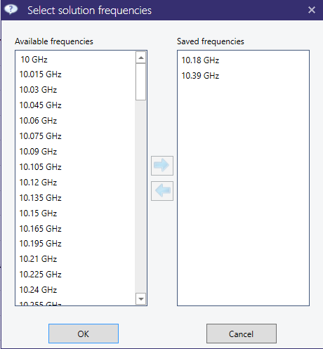
8.4 Solution/Field data saving

When using the default simulation settings, InventSim does not save the information about computed fields. InventSim simply calculates the transfer function between the ports defined in the project. In order to save the fields at user-defined frequencies, move to the simulation settings and the "Solution data" section on the bottom (Fig8.2). Select the "Choose" button and a new window will appear (Fig.8.3) with the list of all simulation frequencies. Select those that are of interest to you.

Remarks:

• • Only if the field information is saved can you evaluate and display the fields or post-process the near fields using the near-to-far field transformation.

• • If the fast-frequency sweep is used in the "Narrowband" mode, the field information is available only at a solution frequency that is set in the fast frequency sweep options.