10 Design Tuning and Optimization

In practice, a single electromagnetic simulation of a complex model is rarely used. Usually a series of computer simulations is performed to optimize the computer model. This is done to achieve the required properties of the structure. InventSim was created to simplify this task by either using manual tuning or the automated optimization schemes. In both cases, one of the most important tasks is the proper structure parameterization using variables, as well as the definition of the design parameters/variables. These variables are called "optimization variables" in InventSim.

10.0.1 Optimization variables

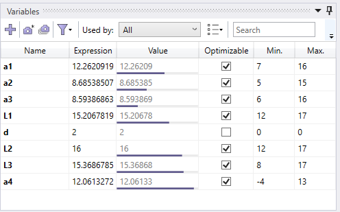
Optimization variables are a special type of variables that is introduced to tune or optimize the model. To change the variable type from a regular to an optimization variable, you need to use the IsOptimizable checkbox in the variable properties. Then you can setup the available range of the variable values. This is the range of the variables that will be then accessed and modified by the optimization/tuning module. Optimization variables are marked with a check-box on the list of variables. The colored line below the value text field corresponds with the relative value of the variable in the range of the allowed values. (Fig. 10.1). Please note that only those variables that have numerical expressions can be made optimizable.

10.0.2 Structure parameterization

Proper structure parameterization is a key part of every design tuning. In general, parameterization should allow you to change the model using the design parameters in a way where each combination of allowed values of the design parameters of the model will remain valid. This, for example, means that no structure will break or unintentionally disconnect from the signal path. In order to achieve the proper parameterization, you can use a combination of variables, equations and relative coordinate systems.

10.1 Design tuning

A unique feature of InventSim is the design tuning module. It allows for fast tuning of the transfer function of the model (e.g. scattering parameters). In order to use the tuning feature, the fast frequency sweep or interpolating sweep must be enabled!

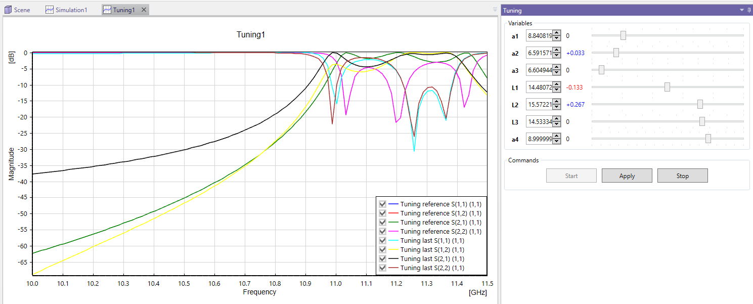
To run the tuning, select the "Tuning" tab and click the "Start" button, Fig.10.2. You can access of the optimization/tuning variables defined in the project in the tuning window. Once the "Start" button is clicked, the solver will simulate the structure. Afterwards, you can modify the values of geometric variables using sliders and see the predicted response of the circuit on the response plot (Fig.10.3). The plot shows both the original response as well as the predicted response which are evaluated for the updated values of variables. The evaluation of this response should not take much time - the plot is updated almost instantly.

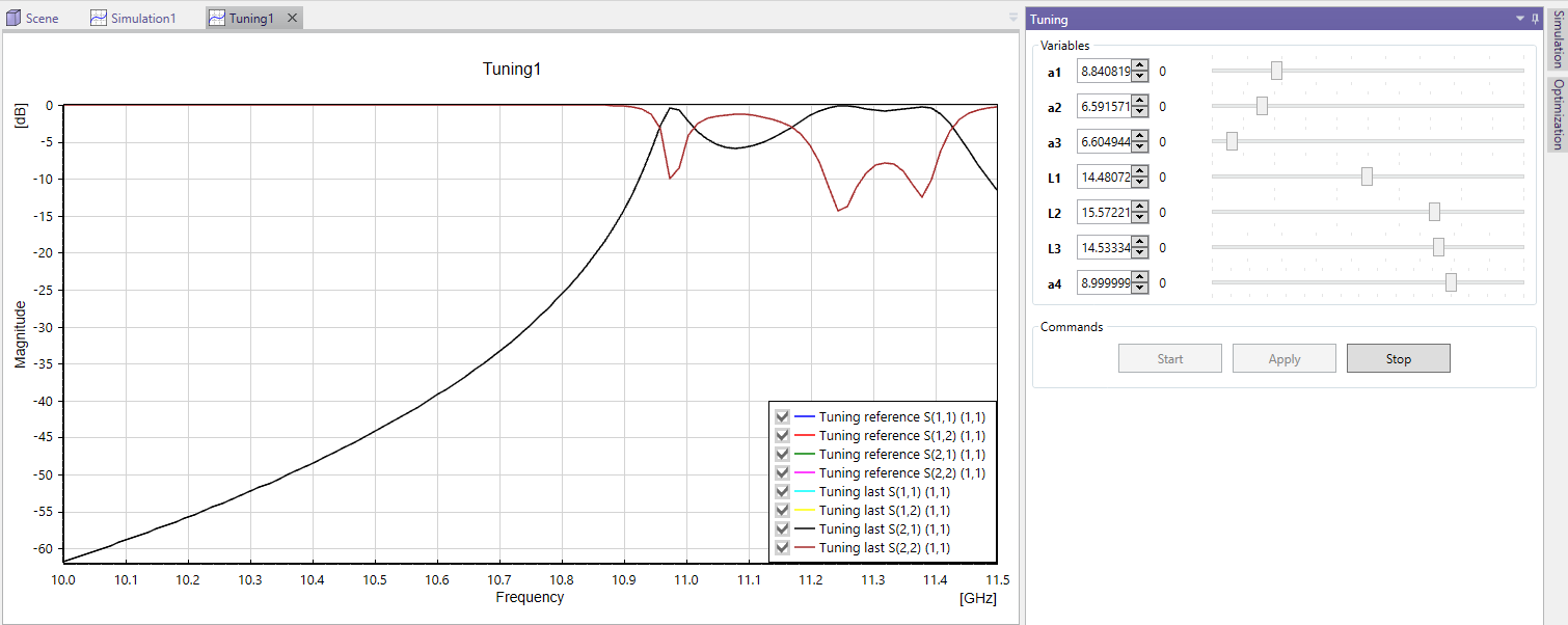
Once the response is satisfactory, it can be validated with the "Validate" button click. The solver will then start the evaluation of the true response of the circuit with a new electromagnetic simulation. Once the simulation is finished, you can continue with the next iteration of the design tuning (Fig.10.4).

10.2 Standard gradient optimization.

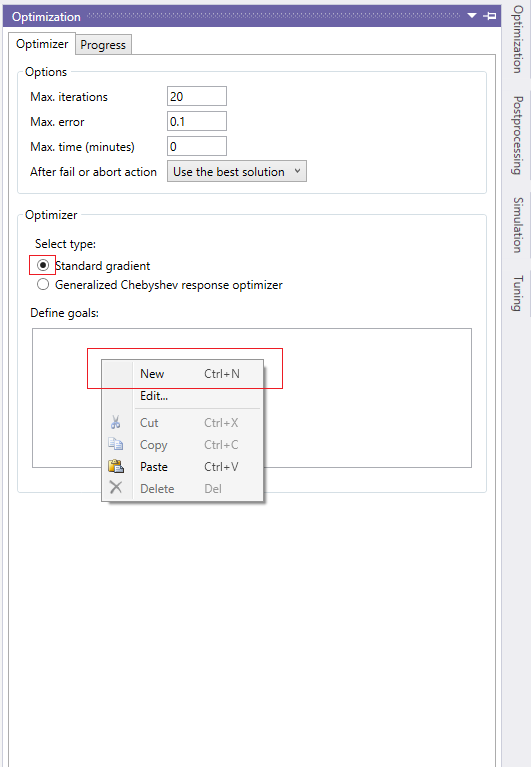
The most fundamental and versatile optimizer available in InventSim is a gradient-based algorithm. In this approach, the user defines the objective function while imposing the requested masks (which specify allowed and restricted regions, defined with inequality operators) on the component’s response. In this context, users can establish multiple objectives based on the frequency domain response of the component undergoing optimization. To add the goal, please right click on the goals list, as shown in Fig.10.5, and then define the goal in a straightforward manner.

Once the goals are set and the optimization variables are defined, the optimization can be started. Please note, that the optimization is allowed only when fast frequency or interpolating sweep is activated.

The optimizer aims to find the best attainable solution but does not guarantee goal achievement. Success depends on various factors, including the definition of the cost function, meshing accuracy and the feasibility of the structure to meet the specified requirements.

10.3 Generalized Chebyshev Cross-Coupled Filter Optimizer / Coupling matrix synthesis

One of the features of InventSim is a built-in software component for optimization of the RF/microwave coupled resonator filters. With this module, you can easily define the requested filter prototype response by using basic filter specifications such as the passband, insertion, loss level and the positions of transmission zeros (Fig.10.6).

Once the desired response is defined by the user and ready, the goal window can be closed. InventSim will save this response as the reference (goal) for the optimization. If the structure is parameterized with optimization variables, you can start the optimization using the "Optimization" button (Fig.10.7). In order to use the optimization feature, fast frequency sweep must be enabled in the project!

The optimizer is then started. It controls the design in a fully automated manner. The algorithms used during optimization involve a zero-pole cost function that usually exhibits fast convergence when filtering structures are optimized. The response sensitivities are computed using mesh perturbation analysis algorithms implemented in our geometry kernel. To speed up computation, mesh deformation can also be used during the optimization process. The response of each iteration is shown on the plot and plots of optimization progress are available. If optimization is stopped, the best solution is taken as as the current value of design variables. The same tool can be used to perform a coupling matrix synthesis for a provided low-pass filter prototype response. Note, the coupling matrix is not needed to perform design optimization!

In the examples folder, you can find the project file ’wg_optimization.ispr’ which demonstrates the efficiency of the filter optimizer on the example of a rectangular cavity waveguide filter design.

Remarks:

• • The filter optimizer usually exhibits fast convergence, as long as the response is feasible to achieve in the model.

• • The optimizer is suited for cross-coupled filter structures for which the response can be described with a rational function. Other filter types, like extracted pole filters, are not supported.

• • As in every other optimization scheme, the convergence of optimization can not be guaranteed.

10.4 Optimization troubleshooting

A crucial factor for successful design optimization in InventSim is a proper parameterization of the 3D model. To achieve maximum efficiency, the topology of the model (i.e. the number of surfaces and edges, along with their relations) should not change within the tuning/optimization process. This consistency allows for efficient geometry processing and the assessment of design sensitivities. If you encounter errors during optimization, they often stem from unexpected changes in the geometry’s topology or the creation of very small edges or surfaces when altering the design variables. In such cases, we recommend thoroughly inspecting your model and resolving any parameterization issues.