9 Postprocessing
Once the simulation is completed, it is possible to perform postprocessing of the calculated field solutions, which includes:
-
• Displaying the calculated transfer function,
-
• Visualization of computed electric and/or magnetic fields,
-
• If the absorbing (radiation) boundary condition is present, transform the near field to the far field and display the radiation pattern as a 2D or 3D plot and evaluate the radiation parameters (gain, efficiency, etc.).

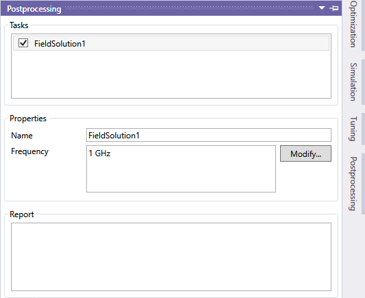
The postprocessing tasks are available in the "Postprocessing" panel on the right side of main InventSim window - Fig. 9.1. With this option you can add, modify and remove postprocessing tasks defined in current project.
Evaluation of the transfer function is a default task in InventSim - no additional postprocessing task is needed to display the transfer function.
9.1 2D Plots of transfer functions
A core functionality of InventSim is calculating the transfer function between ports defined in the project. By default, InventSim computes and displays the transfer function in the form of plots of scattering parameters. If the project does not have a defined plot and the simulation is about to finish, you will need manually add a default plot for computed scattering parameters.
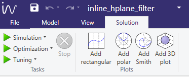

The plot type options is accessible in the "Solution" window located in the upper part of the main application window (the toolbar shown in the picture 9.2). Few plot types are available:
-
• Rectangular. Basic 2D plot with (X,Y) axes.
-
• Smith. Smith chart used to display impedance/admittance parameters.
-
• Polar. Basic 2D polar plot for visualization of radiation patterns.
-
• 3D. 3D plot in spherical coordinate system for visualization of radiation patterns in 3D.
The results of port-driven simulation can be plotted as S,Y,Z, VSWR or group delay parameter plots. For of each set of data series, the user can also apply the additional modifiers, like:
-
• Magnitude
-
• Magnitude in dB
-
• Phase
-
• Real part
-
• Imaginary part
-
• ...
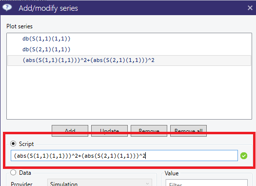
It is also possible to use the data set and invoke the user-defined script, based on mathematical formula provided by the user - overriding the software preset. For example, the power budget \(P\) of two-port network can be calculated based on formula \(P = \mid S_{11} \mid ^2 + \mid S_{21} \mid ^2 \). The example of such definition is shown in Fig.9.5. The list of functions that can be used to define a custom data series via the script functionality is shown table 4.
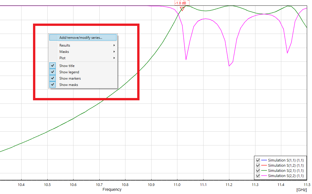
The plot type can be changed from the context menu by selecting "Add/remove/modify series...".
Each of the plotted parameters is represented by a data series and it is plotted as a line. The plot series are listed in the legend on the right side of the plot. The default name for simulation results is "Simulation" with the ID of the port. You can temporarily remove the plot series from the plot by deselecting the checkbox located on the left side of the legend item.
Zooming on the plot is achieved by selecting the region of the plot with the mouse while pressing the left mouse button. To zoom out from the plot, choose "Reset zoom" from the context menu of the plot. Alternatively, exact axes limits can be set in the "Options" panel at the bottom of the plot.
| Symbol | Description |
| ̂ | Power |
| + | Add |
| - | Subtract |
| / | Divide |
| * | Multiply |
| sin() | Sinus |
| cos() | Cosinus |
| tan() | Tangent |
| cosh() | Hyperbolic cosinus |
| sinh() | Hyperbolic sinus |
| tanh() | Hyperbolic tangent |
| conj() | Complex conjugate |
| real() | Real part |
| imag() | Imaginary part |
| phase() | Phase of complex data series |
| mag() | Magnitude |
| ‘ complex() | ? |
| abs() | Module |
| max() | Maximum value of data series |
| min() | Minimum value of data series |
| pow(,n) | Power function |
| log10() | Common (base-10) logarithm |
| log() | Natural logarithm |
| db() | 20log10(\(\cdot \)) |
| db10() | 10log10(\(\cdot \)) |
| ceil() | Smallest following integer |
| floor() | Largest previous integer |
| sqrt() | Square root |
| exp() | Exponential |
| normalize() | Normalize data series to max. value |
9.1.1 Markers
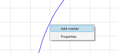
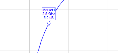
To attach a marker to the current plot, select the data series to which the marker will be added (the series line will be highlighted) and use the context menu (Fig.9.6). Once the marker is added at a specific point of the plot, it can be moved to a different point by using the mouse.
9.1.2 Exporting data.
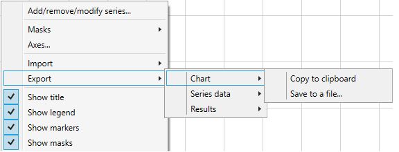
The simulation data can be exported to a file by using the context menu on the plot and selecting submenu "Export ->". The data can be exported on different ways (Fig.9.7):
-
• As a graphic of the active chart window. The available output formats are: .PNG, .GIF, .JPG, .BMP and .TIFF. Using the same context menu, you can also copy the current plot to the clipboard.
-
• As data series to CSV file,
-
• As simulation result file using Touchstone file format.
9.1.3 Zoom/Move/Autoscale 2D plot
To zoom in on the plot area, click LMB on the plot and select the upper corner of the area that needs to be seen in greater detail. Then, move the mouse to the right and down to mark the requested area. To move the plot, use the right mouse button and simply drag the plot.
To restore the view of the plot after the zoom option has been used, click the LMB on the plot area and move the mouse to the right as well as up.
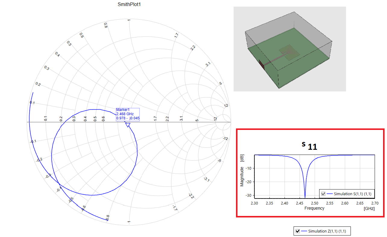
9.2 Smith chart
The admittance/impedance parameters can be plotted on the "Smith" chart. The "Smith" chart can be added using the "Plots" section in the "Solution" toolbar. (Fig. 9.2). Please note that since the electric field formulation is used, we compute the admittance parameters directly, but the reference impedance to transform the Y-parameters to S-parameters is a modal (wave) impedance, applying a relation [9]:
\begin{equation} S = 2 \cdot (I+Y)^{-1} - I \end{equation}
where \(I\) is a unitary matrix. Please also note that in the case of wave ports (non TEM-mode), the characteristic impedance is not unique. Only in the case of lumped ports can we re-normalize the scattering parameters to characteristic impedance and then to 50\(\Omega \) standard. Example of a Smith chart is shown in Fig.9.8.
9.3 Field visualization
InventSim provides near field visualization capabilities which allows to render either scalar (i.e. magnitude of the field) or vector form of the electromagnetic field in Scene panel. The scalar form can be displayed as 3D isosurfaces (surfaces of constant field magnitude) or 2D isolines on a cut plane. The vector form is displayed as arrows which direction represent the direction of the field and length/color representing the E/H field magnitude.
9.3.1 Adding
Visualizations require data calculated in postprocessing stage based on field solution saved for the user-defined frequency points, as described in section 8.4. The necessary postprocessing task can be added by selecting "Add field solution" from the context menu of "Postprocessing" tab in "Simulation" panel. The task is then added with a default frequency set. The frequencies can be changed by clicking "Modify" button and selecting the desired frequency in the dialog window. Please note that the selected post-processing frequency must be defined within the frequency sweep. If the user changes the simulation frequency plan in a way that removes the post-processing frequency point, the simulation will not be executable.
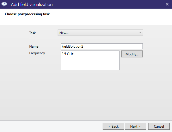
Alternatively, the postprocessing task can be added automatically while adding the visualization. To do so select "Show field" in Scene context menu which will open a wizard window consisting of three wizard pages. The first one allows to choose a data source in a form of a postprocessing task. User can either choose an existing postprocessing task or add a new one with a specified frequency list. As each postprocessing task is executed independently, please make sure to reuse and share existing tasks when creating multiple field plots.
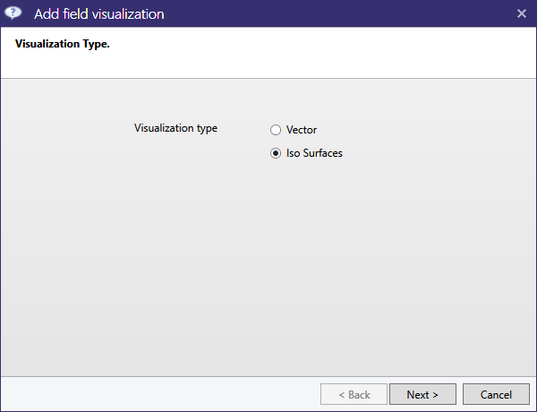
The second page lets choose the visualization type: isosurface/isoline or vector type:
Finally, general visualization parameters are specified i.e. frequency, port and mode of the excitation, field type and coordinate system.
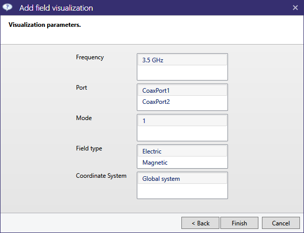
Clicking "Finish" button closes the wizard window and adds postprocessing task as well as field visualization to the project. It also starts postprocessing task calculation and visualization generation task. Once the tasks are finished, field visualization is displayed in Scene. The examples of field visualization are shown in Figures 9.13 and 9.14.
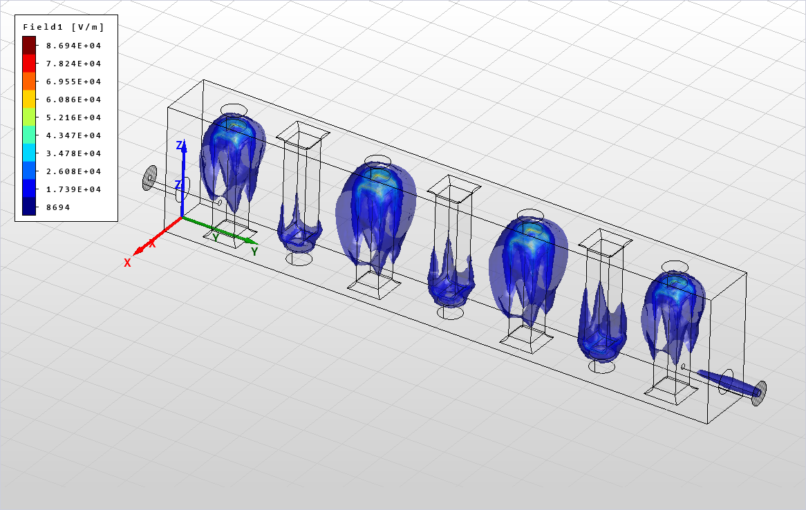
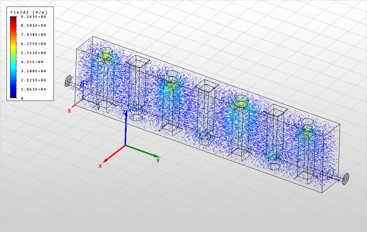
Each field visualization has a corresponding legend displayed on the left part of the screen, as shown in figures above. When isosurfaces/isolines are displayed, the legend shows a set of colors, each representing a field value displayed as a isosurface/isoline. Please note that there is no isosurface/isoline representing neither minimum nor maximum value of the field. In case of vector field visualization the legend shows continuous set of colors as displayed arrows representing field value and direction can have any value, including minimum and maximum values as well.
9.3.2 Parameters
Field visualization have a number of parameters to customize the displayed result. The common set of parameters is:
| General | |
| Name |
Name of the visualization |
| Is visible |
Shows or hides the visualization |
| Object |
Object for which field visualization is generated (not used) |
| Visualization | |
| Postprocessing task |
Name of postprocessing task, the data source of the visualization |
| Color map |
Color map used to color isosurfaces, isolines and vectors |
| Field type |
Electric or magnetic field |
| Coordinate system |
Coordinate system used in iso lines cut plane definition |
| Auto limits |
If true visualization is always displayed based on the current min and max values |
| Max value |
If Auto limits is set to false, this value is used to display visualization |
| Min value |
If Auto limits is set to false, this value is used to display visualization |
| Excitation | |
| Frequency |
Excitation frequency |
| Port |
Excitation port |
| Mode |
Excitation mode |
| Phase |
Excitation phase |
Additionally scalar field visualization have parameters:
| Isosurfaces | |
| Is visible |
Indicates whether to display isosurfaces |
| Count |
The number of isosurfaces |
| Isolines | |
| Is visible |
Indicates whether to display isolines |
| Count |
The number of isolines displayed |
| Colored surface |
If set to true, cut surface will be colored |
| Offset value |
Offset value in the current cut axis in Coordinate system |
| Cut axis |
The axis defining the cut plane |
Vector field visualization have additional parameters:
| Vector field | |
| Scale |
Set scaling factor for displaying the arrows |
| X Count |
The number of sections in X axis |
| Y Count |
The number of sections in Y axis |
| Z Count |
The number of sections in Z axis |
| Is irregular |
If set true, vector positions will be generated randomly |
| Is visible |
Indicates whether the arrows are displayed |
9.4 Radiation patterns
To simulate open structures in InventSim, you should apply the absorbing boundary condition (ABC). This allows the truncation of the computational domain and solving the problem that has a reduced size. Once the simulation is completed and the structure fields are saved for the frequencies defined by the user (look how to define those frequencies in section 8.4), InventSim allows you to calculate the radiating fields in the far field zone using a near-to-far field transformation. In this case, the outer surfaces for which the boundary condition is defined are the source of the external far field. The far field zone distance/radius has to be defined by the user.

You need to add a postprocessing task to calculate the radiation patterns. It can be done in two ways:
-
• Selecting the "Postprocessing" tab in the "Simulation" options window and using the context menu to add a new task,
-
• Using the context menu of the 3D geometry modeler and selecting the "Show radiation" item.
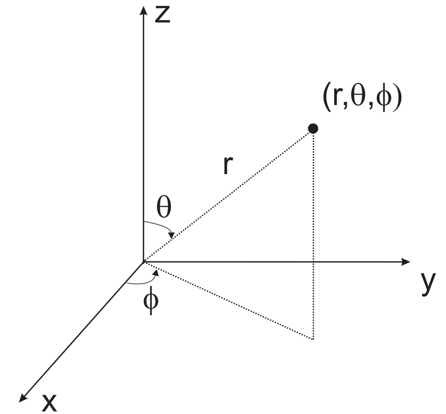
Definition of the near-to far field task requires you to provide the observation angles in a spherical coordinate system (Fig. 9.15).
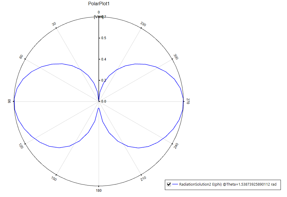
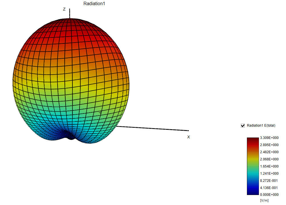
A set of the observation angles is defined for both \(\theta \) and \(\phi \) coordinates with a minimum and a maximum angle value and a number of \(N\) observation points that are uniformly distributed within this range (Fig.9.16). You can define a task of computation of the fields for a single cut (for constant \(\theta \) or \(\phi \) angles, with \(N\)=1) and create a plot in rectangular or polar coordinates (Fig.9.17) You can also compute the fields with both varying angles \(\theta \) and \(\phi \). The latter allows you to compute a 3D plot of radiation patterns, as shown in Fig 9.18.
9.4.1 Near-to-far field transformation
The near-to-far field transformation is implemented using the approach that is described in [27]. In the far field region (in the radial distance \(R > \frac {2D^2}{\lambda }\), where \(D\) is the largest dimension of radiation source), the electric field components in spherical coordinate system can be evaluated from near-electric and magnetic fields using these relations:
\begin{equation} E_{\theta }(r) = - \frac {jk_0 e^{-j k_0 r} }{4 \pi r } (L_{\phi } + Z_0 N_\theta ) \end{equation}
\begin{equation} E_{\phi }(r) = \frac {jk_0 e^{-j k_0 r} }{4 \pi r } (L_{\theta } - Z_0 N_\phi ) \end{equation}
where \(\vec {L}(r)\) and \(\vec {N}(r)\) are computed as integrals over surface \(S\) that encloses the source of the radiation:
\begin{equation} \vec {N}(\hat {r}) = \iint _S \vec {M}(r') e^{j k_0 r' \cdot \hat {r} } dS \end{equation}
\begin{equation} \vec {L}(\hat {r}) = \iint _S \vec {J}(r') e^{j k_0 r' \cdot \hat {r} } dS \end{equation}
and
\begin{equation} \vec {J} = \vec {n} \times \vec {H} \end{equation}
\begin{equation} \vec {M} = - \vec {n} \times \vec {E} \end{equation}
In this notation, \(\hat {r}\) is a unitary vector pointing to the observation point, \(r'\) is a vector of source location and \(\vec {n}\) is a vector that is normal to the surface S. According to the electromagnetic field theory, the radial components of the field vanish in the far field zone and only the transverse (\(\theta \), \(\phi \)) field components are present.
The computation of the far field is done internally. You need to specify the observation points (using the spherical coordinate system). Once the fields are computed, they can be displayed either as a 2D or a 3D plot.
Please note that the near-to-far field transformation might be a computationally intensive process.
9.4.2 Radiation parameters
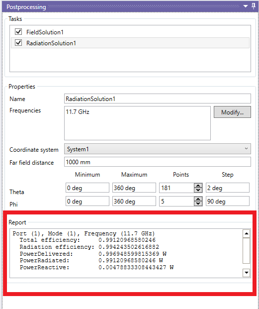
When the radiation task is defined and solved, InventSim automatically calculates selected antenna/radiation parameters and reports them in a post-processing task panel, as shown in Fig.9.19. The report includes:
-
• Total radiation efficiency - ratio of the total power radiated by a component to the net power delivered by the source. The source is normalized to available power equal one Watt (1W).
-
• Radiation efficiency - ratio of the total power radiated by a component to the net power accepted by the antenna from the source.
-
• Power delivered to component.
-
• Power radiated (real part of complex-valued radiated power.)
-
• Power reactive (imaginary part of complex-valued radiated power.)
9.4.3 Antenna gain
Antenna gain is defined as the ratio of the intensity, in a given direction, to the radiation intensity that would be obtained in the power accepted by the antenna were radiated isotropically. The radiation intensity corresponding to the istropically radiated power is equal to the power accepted (input) by the antenna divided by \(4\pi \) (definition by C.A. Balanis, "Antenna Theory: Analysis and Design".):
\begin{equation} Gain = 4\pi \frac {U(\theta , \phi )}{P_{in}} \end{equation}
where \(U(\theta , \phi )\) is a radiation intensity
\begin{equation} U(\theta , \phi ) = \frac {R^2}{2\eta } \cdot \| E(\theta , \phi ) \|^2 \end{equation}
with \(R\) given as a far field zone radius, and \(E(\theta , \phi )\) far-field zone electric field of antenna, and \(\eta =120\pi \) is free space impedance. With this notation, the antenna gain can be evaluated in InventSim using an equation
\begin{equation} Gain = 4\pi R^2 \frac { \| E(\theta , \phi ) \|^2}{2\eta \cdot P_{in}} \end{equation}
Assuming \(P_in = 1W\), and \(R=1m\) (default values in InventSim), one gets:
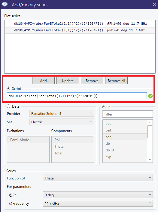
\begin{equation} Gain = 4\pi \frac { \| E(\theta , \phi ) \|^2}{2\eta } \end{equation}
The formula can be then directly implemented in InventSim plot with a script functionality, as shown in Fig.9.20.