7 Meshing options

Mesh generation is a crucial part of every finite element simulation. Its task is to construct a discrete representation of a modeled geometry. In InventSim, we use a tetrahedral grid in order to be able to model complex, arbitrarily shaped geometries.

To generate a mesh, InventSim uses the third party software Netgen [12, 13] that generates good-quality, second-order grids. The mesh influences the accuracy of simulation results in several ways:

• • The mesh is a discrete representation of original geometry. The meshing process can introduce a discretization error, especially if curved boundaries are present in the structure. In InventSim, to achieve a better representation of curved shapes, we use a second order mesh, where the element edges are second order curves (Fig. 7.1).

• • In order to properly model the field behavior, the mesh needs to be adequately fine. In general, it is recommended to set the initial, vglobal maximum mesh edge length as \(\frac {\lambda _{min}}{5}\), where \(\lambda _{min}\) is the wavelength at the maximum simulation frequency. However, in regions that exhibit strong field variation, you may need to refine the mesh. In InventSim, you can use adaptive mesh refinement to improve the accuracy of the results.

• • Poor-quality, needle-like or nearly flat tetrahedral elements with high aspect ratio would result in deterioration of main matrix conditioning number. This might cause problems during the solution phase, especially if iterative solvers are used.

The meshing options can be found in the "Simulation" tab on the right side of the main GUI window (Fig. 7.3). The window is divided to two sections: global mesh and adaptive meshing options.

7.1 Global mesh settings

The process of meshing creates a tetrahedral volume mesh and a triangular surface mesh, based on the geometrical model of the structure. A single mesh cell size as well as the global distribution of cell sizes are determined by several factors.

Default behavior of the meshing is controlled by global options located in the "Global parameters" section of the "Mesh" tab. These options include:

• • Maximum mesh size - the maximum edge length in the mesh (global). This setting determines uniform refinement of the mesh.

• • Segments per radius - defines the number of sections into which the curved edges will be divided. This determines how well the round edges will be approximated.

• • Segments per edge - defines the number of sections into which the straight edges will be divided.

• • Grading - specifies the amount of variation in the size of adjacent cells. Normal is the default value, which allows a certain degree of local mesh refinement. Low setting value results in a more uniform mesh, while High setting generates highly non-uniform mesh.

7.2 Adaptive meshing

A typical structure consists of regions where the mesh needs to be refined, while at the same time there are other regions where the mesh can be coarse without sacrificing the accuracy. It is difficult to predict the areas where the finer mesh is required, therefore the adaptive meshing procedure should be used. The repeating procedure refines the mesh locally in order to improve the accuracy of the results.

The accuracy is tested at a set of frequency points by comparing the magnitudes of scattering parameters calculated at those points. The procedure stops when a specified number of consecutive simulations report the results differing by less than a specified value.

The adaptive meshing is set up in the "Mesh" tab of the "Simulation" panel. The procedure can be switched on and off by selecting "Use adaptive meshing" checkbox. The frequencies at which the accuracy is tested are defined in a fashion similar to setting the simulation frequencies (please see "Frequency sweep simulation" chapter for details). The main parameters of the adaptive meshing are:

• • Accuracy - the maximum difference between the magnitudes of scattering parameters.

• • Mesh size increase - the fraction of the mesh vertices that will be designated for refinement. The higher the value, the greater the problem size in consecutive iterations.

• • Maximum iterations - the total number of iterations.

• • Converged iterations - the number of iteration that allow the error to be smaller than "Accuracy" after which the adaptive meshing will converge.

In practice, your experience and knowledge about field solutions predicted within the structure might be used to make the initial mesh as good as possible. This would limit the number of adaptive mesh iterations and therefore reduce the simulation time. To refine the mesh locally, you can use "Local" mesh parameters.

7.2.1 Enabling adaptive mesh frequencies

The adaptive mesh refinement is disabled by default. To enable it, you need to click the "Adaptive meshing" checkbox and add at least one (possibly more) frequency point. The convergence of the adaptive mesh refinement will be tested at this point(s). To add a frequency, please click the right mouse button on the "Frequencies" window to use the context menu. Then select "Add" and define the start, stop and a number of frequency points - usually this will be done on just one or two points to reduce the simulation time. Here are the recommendations:

• • In non-resonant, transmission-line structures define the frequency as the highest frequency of simulation,

• • In resonant structures, like filters, define the frequency close to the passband or within the passband, since the field variations are at the highest close to the resonance,

• • If a structure has multiple resonances with different modes or located in a different part of the domain, then you can define more than one frequency close to the resonant frequencies. It is done to properly model field variations at the resonance.

7.2.2 Example

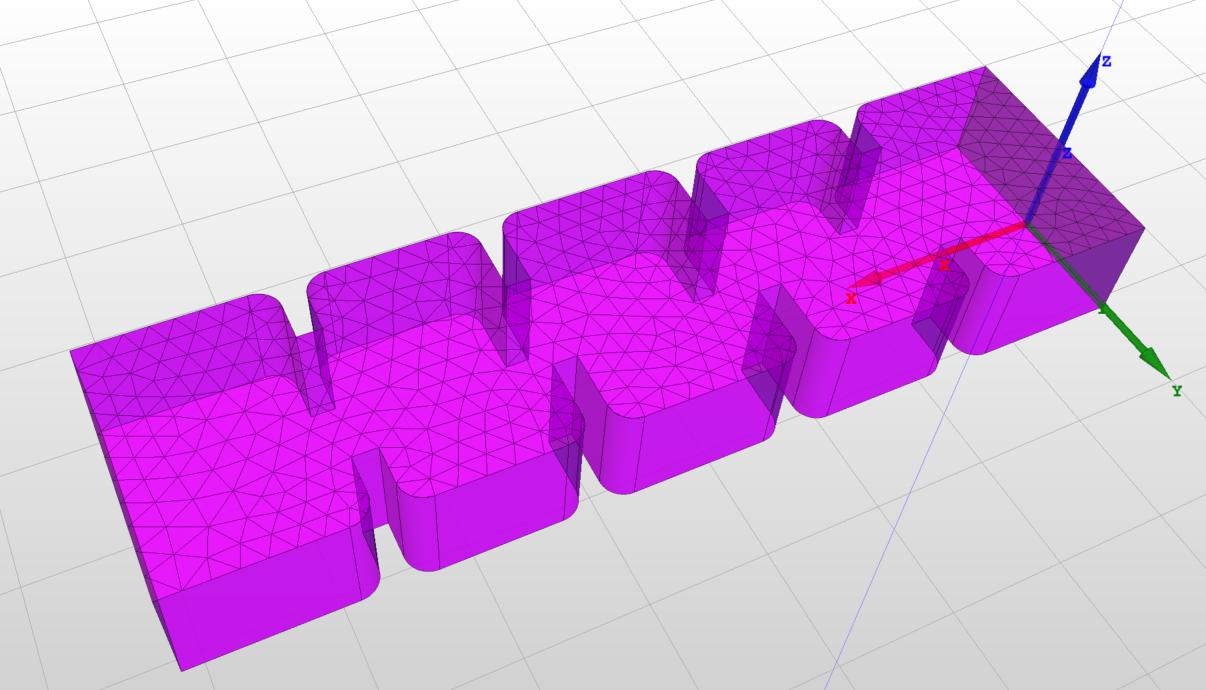
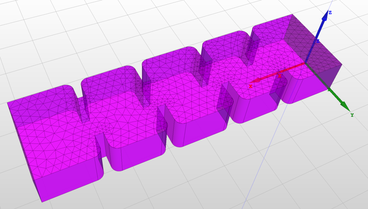
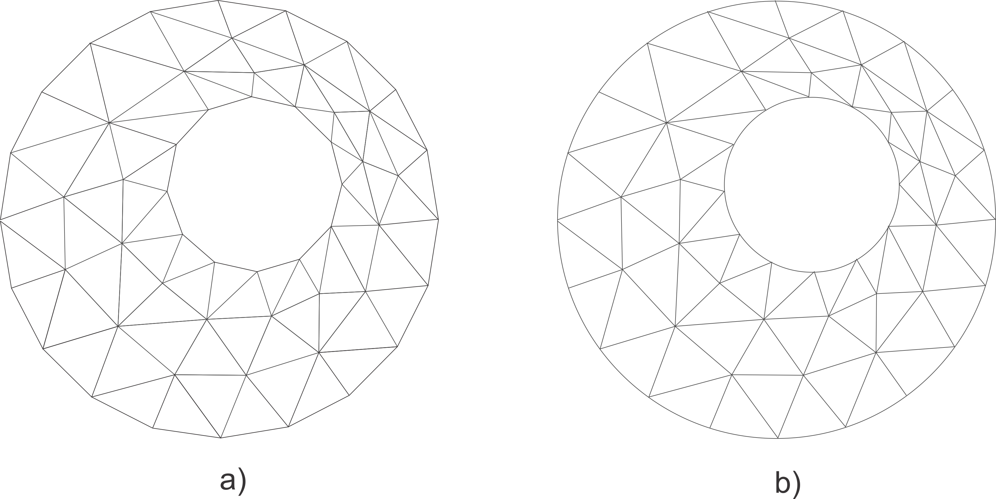
Fig. 7.4 presents an example of an application of adaptive mesh refinement using a simple, H-plane waveguide filer. When comparing the uniform mesh with the adaptively refined mesh, it is noticeable that the adaptive mesh refinement algorithms implemented in InventSim allow you to generate a mesh that can represent the fields in the structure in a positive way: the most important areas that have a high field variation will have a much smaller mesh size.

7.3 Mesh refinements

Another tool that allows control of mesh behavior is Mesh refinements. It allows to restrict mesh cell size in selected regions of space in order to override global mesh settings. It can be used either in conjunction with Adaptive meshing or instead of it, depending on the application and the user’s understanding of the structure field behavior.

The local meshing behavior can be controlled by introducing one or more Mesh refinements to the project. Each of the refinement defines a set of rules on how to restrict mesh cell size. These rules, along with global mesh parameters, are passed to the mesher during meshing phase. Each rule consists of three conceptual parts:

[parsep=2pt]

• 1. Objects - in conjunction with the next part, defines region(s) in 3D space where mesh size would be restricted. SimObjects are used for the user’s convenience to define regions in space.

• 2. Relation - defines which topological part(s) of Objects should be used to determine region(s) of 3D space. The possible choices are listed below and its results depend on SimObject type.

  [parsep=1pt, topsep=1pt]

  • • Inside, on surface and edges

  • • On surface and edges

  • • On edges

• 3. Maximum length - defines the maximum size of mesh cell in length units.

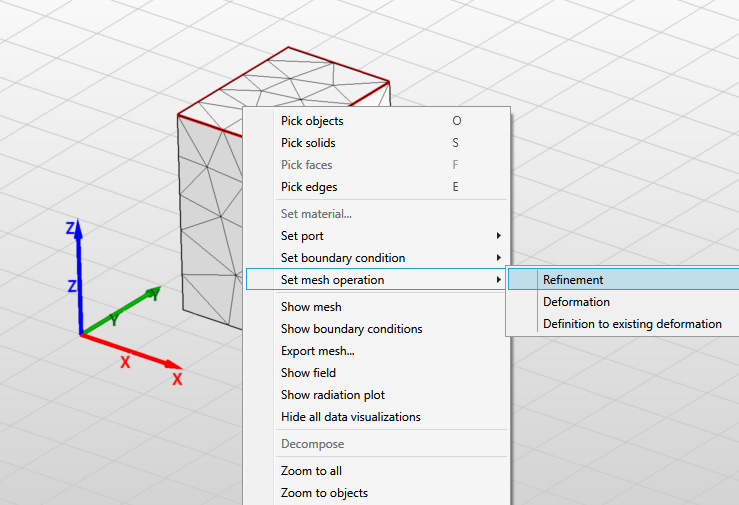
To add a mesh refinement, select the desired solid or a face, open context menu and select "Set mesh operation->Refinement" (Fig. 7.5). The new mesh refinement will be added to the project tree with the following list of parameters:

[itemsep=2pt, parsep=2pt]

• • Name: the name of the refinement.

• • Is enabled: indicates whether the refinement is enabled or not.

• • Maximum length: maximum mesh cell size.

• • Relation: sets how the refinement will be applied to the selected objects.

• • Objects: list of objects on which the refinement is set.

To delete the mesh parameter, first select it in the project tree and then choose "Delete" from the context menu.

If multiple mesh refinements are defined on the same region(s) of space the most restricting parameter will be in effect i.e. the one with the smallest "Maximum length" value. No error nor warning will be shown.

Mesh refinements can also be set on SimObjects which have "Calculate" flag off. Using such a feature user can define an arbitrary region in space which exhibit a desired meshing behavior but does not introduce any geometrical entities into the simulation domain.

7.3.1 An Example

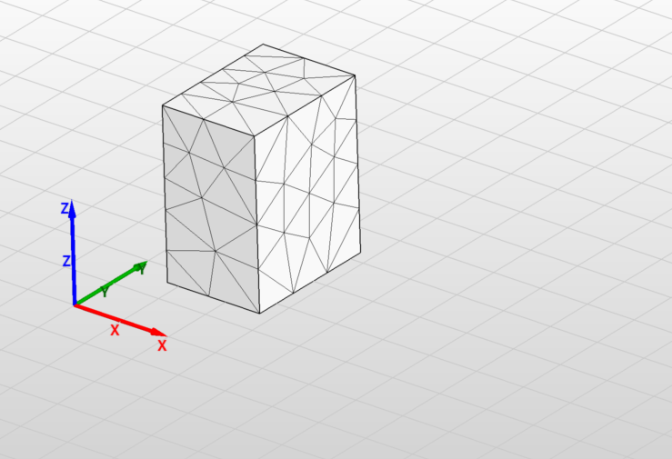
In this example, the structure consists of a simple box sized 5mm x 8 mm x 10mm. The box is discretized with a uniform mesh that has an edge length equal to 3mm, as shown in Fig. 7.5. To refine the mesh on the upper surface, you need to select this surface, then select the "Set mesh parameter" option in the context menu. A new position will appear on the project tree. It is added in the "Meshing" section - it allows you to enter the maximum edge length. If you input 0.8mm, you will get a non-uniform mesh as shown in Fig. 7.5.

7.4 Mesh morphing

The simulation with the finite element method requires a discrete representation of the model using a mesh. The mesh has to be generated every time the model changes - i.e. the geometrical structure dimensions are modified. Common practice in most simulation software tools in this case is to generate the mesh from scratch. Even if the geometry change was comparably small and localized in a small part of the model, the mesh is re-generated for whole structure. Such an approach has several disadvantages [28]:

• • Mesh generation is a time consuming procedure, especially when adaptive mesh refinement is involved.

• • Re-meshing noise can be observed, this means that the model geometry change is continuous, while the change of model response is not continuous.

• • During the solution phase, all data from the previous simulation is lost and the solver starts from scratch.

In InventSim, mesh morphing algorithms are implemented to eliminate those issues. Mesh morphing allows you to modify the existing mesh and move mesh nodes to fit the modified model. As a result, the mesh topology does not change: what changes is only the locations of mesh nodes.

In general, InventSim can morph the mesh of arbitrary, user-defined 3D geometry. There is a restriction though: the modified geometry should have the same topology as the original - i.e. number of the faces and the edges and their connections should remain the same.

Mesh morphing can be used during optimization and tuning. It can also be invoked by the COM interface.

7.4.1 Using COM to morph a mesh

InventSim can be used to perform mesh morphing of a 3D model without further simulation. In order to generate a morphed mesh for a modified geometry, please follow these steps:

• • Load and simulate the project to generate the mesh for initial geometry. The 3D model should be parameterized with variables - only optimization variables can be changed during mesh morphing. Important: the current mesh must correspond with actual model geometry!

• • Connect to the COM server, for example using Matlab/Octave, as shown in Section "COM Interface".

• • Load the set of current values of optimization variables using the COM function:
  x0 = App.ActiveProject.Variables.GetOptimizableVariableValues();

• • Provide the vector of modified variables x1.

• • Obtain reference mesh:
  refMesh = app.ActiveProject.Simulation.GetMesh();

• • Execute mesh morphing using COM method:
  morphedMesh = App.ActiveProject.Simulation.GetMorphedMesh(refMesh, x0, x1, 0);
  Modified mesh is returned by the method.

• • Optionally, restore the original values of variables with this method:
  App.ActiveProject.Variables.SetOptimizableVariableValues(x0);

To repeat the simulation using the morphed mesh, set OverrideMesh property of Simulation with the reference to the morphed mesh and start simulation:
App.ActiveProject.Simulation.OverrideMesh = morphedMesh;
App.StartSimulation();

7.5 Shape deformations

The use of additive manufacturing (AM) technology (also known as 3D printing) to fabricate high-frequency components has been increasing in popularity in recent years. AM allows for the production of complex 3D structures of almost arbitrary shapes, with user-defined surface curvatures. This flexibility in model complexity is a great advantage over established technologies, as the limitations of conventional techniques such as CNC milling no longer apply. In many cases, AM permits the production of a model that would not be achievable using other manufacturing methods. In this context, AM is a key enabling technology that opens up new possibilities to RF & microwave engineers.

However, in order to take advantage of this design flexibility, the limitations of the CAD tools used in the industry need to be overcome. These limitations stem from the fact that virtually all CAD software used for high-frequency electronic design relies on the constructive solid geometry (CSG) approach. CSG is the prevailing paradigm for the 3D modeling of electromagnetic structures. It is based on using a set of simple, predefined geometrical primitives—such as boxes, cylinders, and cones—and applying to them Boolean operations, such as union, subtraction, and intersection, or shape modifications with edge filleting or chamfering. Alternatively, arbitrarily shaped surfaces based on parametric, equation-based objects can be used, but this is cumbersome and difficult to use. The design of more complex geometrical models—such as those with unconventional twisted or bent shapes—is very challenging in this approach. For decades, the CSG approach has been regarded as satisfactory, as design was limited by the available manufacturing technologies, such as CNC milling. This has now changed with the widespread availability of repeatable and accurate 3D printing.

Therefore, to enable the design of microwave components with truly arbitrary shapes, the solution available in InventSim is to empower CSG-based 3D solid modeling tools with a free-form shape deformation technique.

Shape deformation can be treated as an additional step in the design process. It can be performed on objects created initially with CSG. The basic principle of shape deformation is to define a set of points around the object that will control the deforming operation. The deformation is then begun by shifting some of these control points to certain new coordinates, and a vector displacement field is constructed using these displacements. The original structure is then mapped according to this smooth displacement function. The deforming operation can be performed on 3D objects represented by a surface or volume mesh. In InventSim, we consider a tetrahedral mesh used in 3D FEM.

7.5.1 Shape deformation with RBFs

Shape deformation feature in InventSim is implemented using an interpolation scheme based on radial basis functions (RBF), as reported in [29, 30, 31, 32]. In general, a RBF is a real-valued function \(\varphi \) whose value is only determined by the distance from the origin, so that \(\varphi (\boldsymbol {x}) = \hat {\varphi }(\| \boldsymbol {x} \|)\). The principle of the reshaping operation is represented in general by a mapping function \(\mathcal {D}\):

\begin{equation} \begin{split} \mathcal {D}(\boldsymbol {x}) : \mathbb {R}^3 \rightarrow \mathbb {R}^3 \\ \boldsymbol {x} \mapsto \mathcal {D}(\boldsymbol {x}) = \boldsymbol {x} + \boldsymbol {d}(\boldsymbol {x}) \end {split} \end{equation}

In this notation, \(\boldsymbol {d}(\boldsymbol {x})\) can be interpreted as the deformation field applied to the 3D model. In the case of RBF-based deformation, this takes the following form:

\begin{equation} \boldsymbol {d}(\boldsymbol {x}) = \sum _{i=1}^{{N}} \boldsymbol {\gamma _i} \varphi (\| \boldsymbol {x} - \boldsymbol {x_{i}} \|) + p(\boldsymbol {x}) \end{equation}

where \(N\) is the number of control points defining the deformation, \(\boldsymbol {\gamma _i}\) are the weights corresponding to the radial basis functions \(\varphi \) defined at the positions of the control points \(\boldsymbol {x}_i\) (in 3D \(\boldsymbol {x_i} \in \mathbb {R}^3, \boldsymbol {x_i} = [x_i,y_i,z_i] \)), and \(p(\boldsymbol {x})\) is a low-order polynomial (optional).

To perform the deformation, the mapping operation \(\mathcal {D}\) needs to be specified. The first step is to define a set of \(N\) control points and their displacements, which indicate the direction and value of the offset. Next, a certain type of RBF with its parameters (e.g., radius, exponent) is selected: the choice of basis function affects the manner in which the mesh points are interpolated to match the new positions of the control points.

There are many different RBFs commonly used for multivariate function interpolation, six of which are implemented in InventSim:

• • Gaussian spline:

  \begin{equation} \varphi (\|\boldsymbol {x}\|) = \exp ({-(\frac {\|\boldsymbol {x}\|}{r}})^2), \end{equation}

• • multi-quadratic biharmonic spline:

  \begin{equation} \varphi (\|\boldsymbol {x}\|) = \sqrt {\|\boldsymbol {x}\|^2 + r^2}, \end{equation}

• • inverse multi-quadratic biharmonic spline:

  \begin{equation} \varphi (\|\boldsymbol {x}\|) = \frac {1}{\sqrt {\|\boldsymbol {x}\|^2 + r^2}} \end{equation}

• • thin plate spline:

  \begin{equation} \varphi (\|\boldsymbol {x}\|) = \left (\frac {\|\boldsymbol {x}\|}{r}\right )^k \ln \frac {\|\boldsymbol {x}\|}{r} \end{equation}

• • Beckert-Wendland C2 basis:

  \begin{equation} \varphi (\|\boldsymbol {x}\|) = \left ( 1 - \frac {\|\boldsymbol {x}\|}{r}\right )^4 + \left ( 4 \frac {\|\boldsymbol {x}\|}{r} + 1 \right ) \end{equation}

• • polyharmonic spline:

  \begin{equation} \varphi (\|\boldsymbol {x}\|) = \begin{cases} (\frac {\|\boldsymbol {x}\|}{r})^k \quad & \text {if}~k = 1,3,5,...\\ (\frac {\|\boldsymbol {x}\|}{r})^k \ln (\frac {\|\boldsymbol {x}\|}{r}) \quad & \text {if}~k = 2,4,6,...\\ \end {cases}, \end{equation}

where \(r\) and \(k\) are the radius and power of the RBF, respectively. A linear equation system is then solved to find the unknown weights \(\boldsymbol {\gamma _i}\) given the coordinates of the original and displaced control points [31]. The matrix representation of this equation system is as follows:

\begin{equation} \boldsymbol {\Phi }\boldsymbol {\gamma } = \boldsymbol {B} \end{equation}

where \(\boldsymbol {\gamma }\) is the weight matrix of dimension \(N\times 3\), corresponding to \(N\) control points defined in a 3D coordinate system. \(\boldsymbol {\Phi }\) is an \(N\times N\) matrix containing RBF values computed for the Euclidean distances between the corresponding control points, \(\boldsymbol {\Phi _{i,j}} = \varphi (\| \boldsymbol {x_{i}} - \boldsymbol {x_{j}} \|)\), and \(\boldsymbol {B}\) is an \(N\times 3\) right-hand side matrix with the new (displaced) coordinates of the control points. The system is dense, symmetric, positive definite, and its conditioning depends on selected RBF and control points distribution. Once the weights are computed, the deformation field \(\boldsymbol {d}(\boldsymbol {x})\) is constructed and can be applied to smoothly move all the mesh points of a 3D object. It can be seen that the mapping function can be easily defined with a limited number of control points, and then applied to create complex 3D objects. The computational cost of the deformation is also not significant, as the size of the linear problem to be solved is usually small.

7.5.2 Example: deformation of a rectangular waveguide

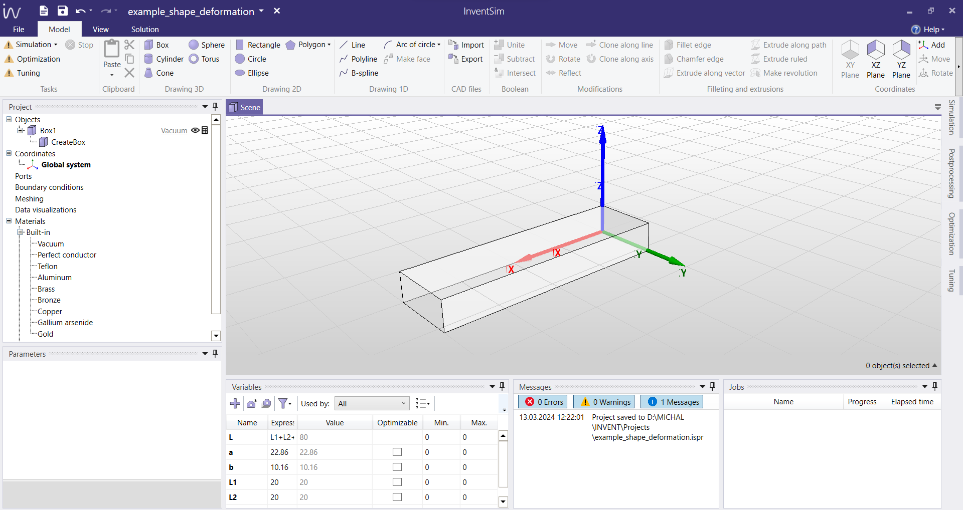
To illustrate the operation of this framework, a simple example of creating a smooth-profile rectangular waveguide filter is presented. First, a basic structure is created using constructive solid geometry: here, a section of a standard WR-90 rectangular waveguide is defined, as shown in Fig. 7.6.

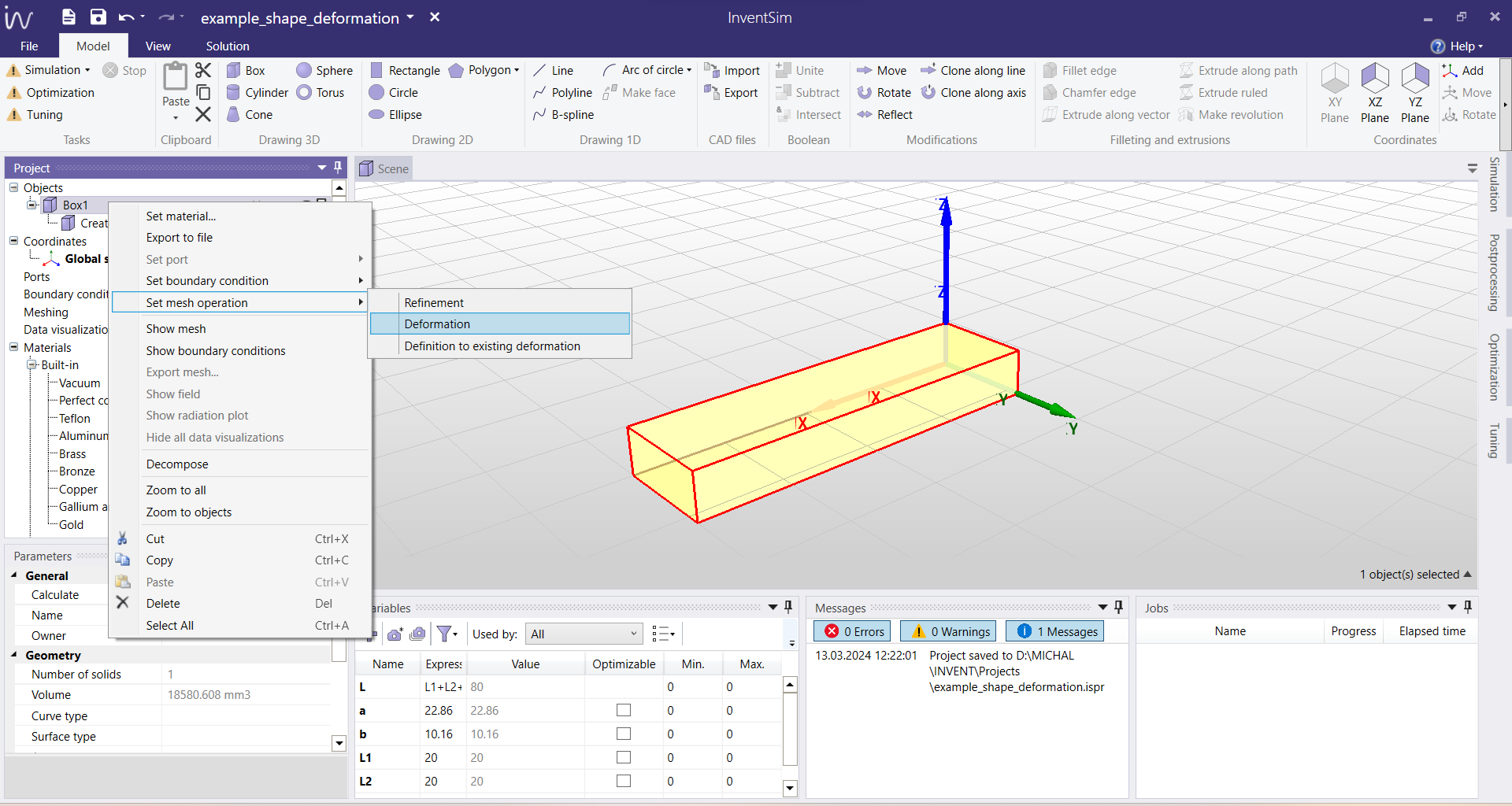
In order to alter the geometry of this structure by shape deformation, a number of control points need to be selected around it. In this example, the control points are defined on a box enclosing the waveguide section. You can do it by creating a new shape deformation definition, by choosing the option "Set mesh operation > Deformation" upon right-clicking on the chosen object, as shown in Fig. 7.7. You can define more than one shape deformation in a single project, but they will be considered as separate operations. If you want to add multiple definitions to a single deformation (i.e., multiple lists of control points to be considered during the same operation), you can choose the option "Set mesh operation > Definition to existing deformation", and add another list of control points to your existing mesh deformation.

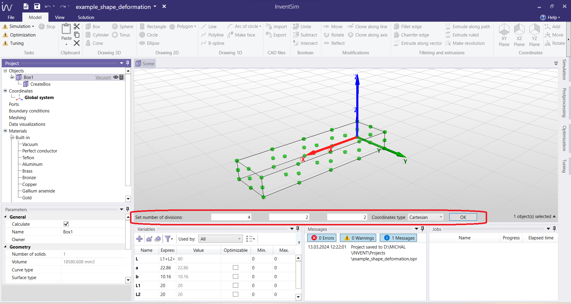
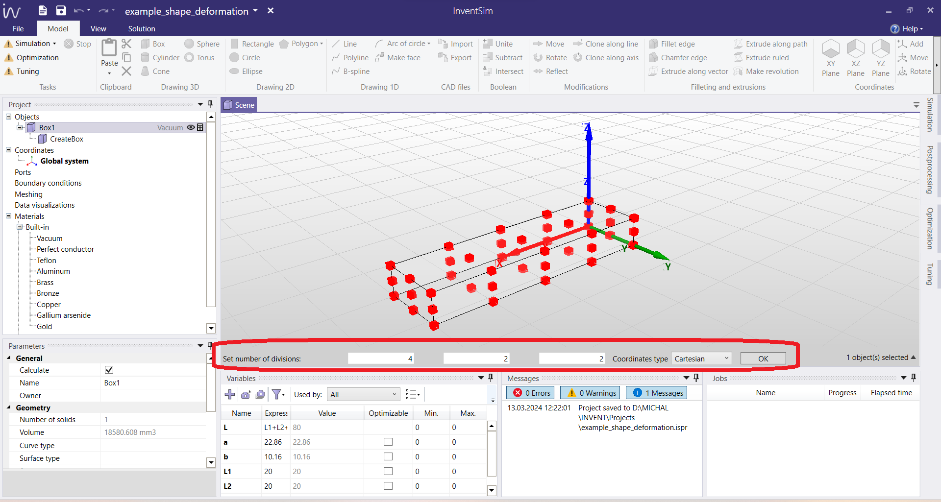
After choosing the option to create a new mesh deformation, an exemplary set of control points is generated automatically around the chosen object, as shown in Fig. 7.8. You can manually change the auto-generated list by selecting the number of divisions, e.g. in each of the three directions defined in Cartesian coordinates: X, Y, and Z. You can modify these points or add more control points afterwards. To be able to modify the auto-generated points, they need to be selected at this point, as highlighted in Fig. 7.9. You can either select each point by clicking on it manually, or select them all by using the key combination "Ctrl" + "A".

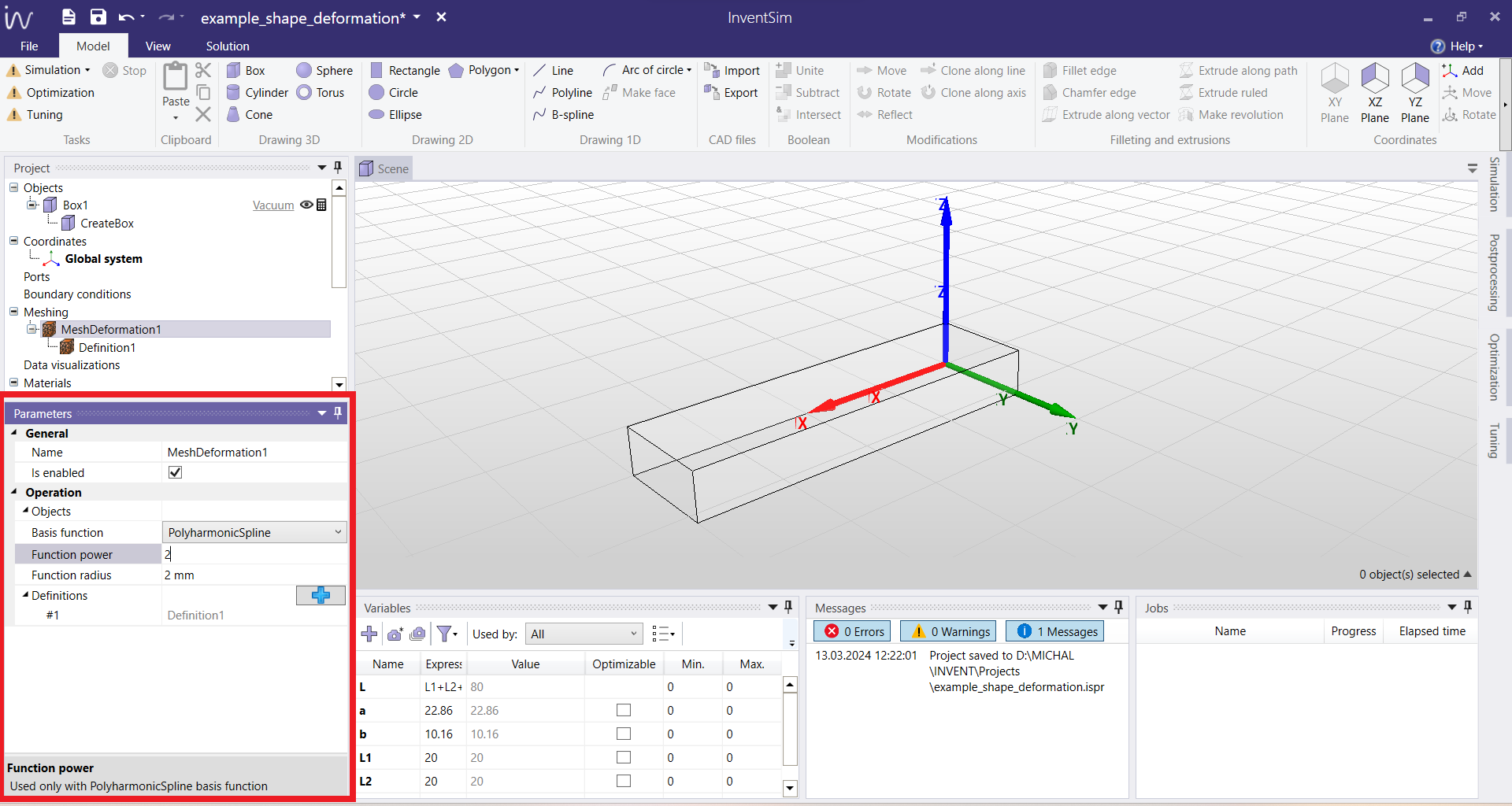
Upon successful creation of the mesh deformation definition, you can find it in the Project tree under Meshing > MeshDeformation1. When selected, you can access its parameters, as shown in Fig. 7.10. From there you can choose the radial basis function to be used in the interpolation, and define its parameters, such as function power and function radius, as was described above in Section 7.5.1. If more than one control points definitions were created, they can all be found under their respective mesh deformation in the Project tree. In this example, there is only one, Definition1, which is linked to MeshDeformation1.

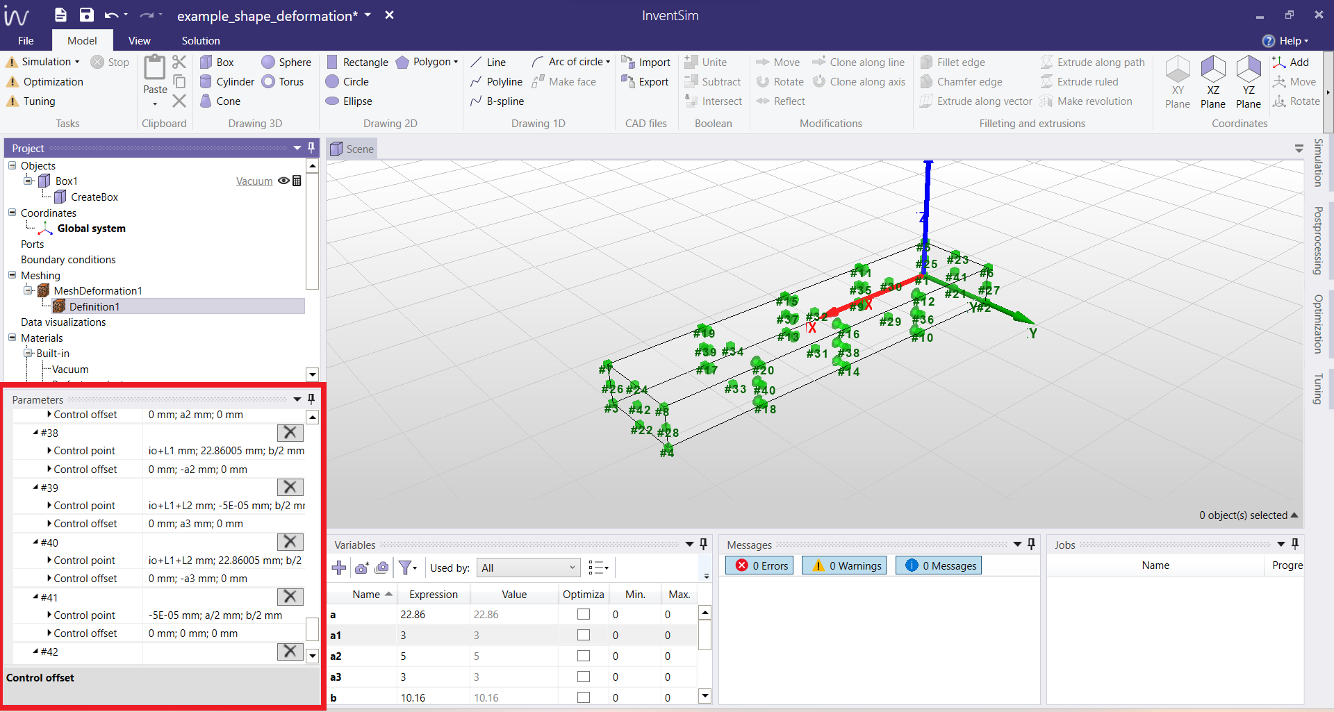
The list of control points and their displacements can be accessed and controlled by choosing the respective Definition (in this example, Definition1). After choosing this option in the Project tree, the user can access the list of control points, as shown in Fig. 7.11. You can edit the coordinates (position) of each point, as well as assign a displacement (offset) to define their movement to a new position. When a non-zero offset is defined, the displacement vector, depicted by a green arrow, becomes visible in the graphical user interface, as in Fig. 7.11. The original structure is deformed depending on the number of control points and the direction of their offsets.

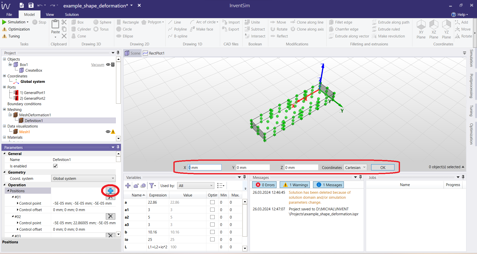
It should be noted that the shape deformation scheme does not limit the number of control points. More complex deformation schemes can easily be employed by adding more control points with movement in arbitrary directions. You can easily add a new control point to an existing deformation by clicking the "+" button located at the heading of the respective Definition containing the list of control points, as presented in Fig. 7.12.

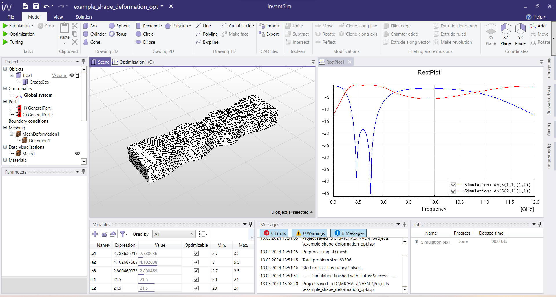
Finally, when the shape deformation parameters and the control points are properly defined, the deformation will be performed during each EM simulation: the deformation is applied to the 3D mesh, just after the mesh generation process. To observe the effect, an EM simulation needs to be run for the project. The parameters used to define the positions and offsets of the control points can be project variables, and they can be used for Tuning and/or Optimization. In this example, a simple squeezing operation was defined for the basic rectangular waveguide section, and the project was optimized to receive a bandpass response, as shown in Fig. 7.13. After the simulation is complete, you can see the deformed 3D mesh by making it visible (right-clicking on the object and choosing the option "Show mesh").