5 Material definitions

A core part of electromagnetic field simulation is the definition of electric properties of materials for all 3D objects defined in the structure. In InventSim, you can use several different types of materials, i.e.:

• • Isotropic, frequency independent dielectric

  • – Lossless

  • – Lossy, with provided loss tangent

• • Isotropic, frequency-dependent dielectric

  • – Debye model

• • Bulk conductors with provided conductivity \(\sigma \)

• • Gyromagnetic materials described with Polder tensor

The list of materials is shown in the project tree window, Fig.5.1.

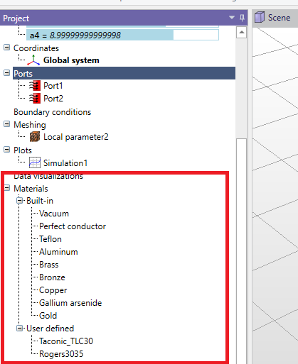
There are several predefined materials available:

• • Vacuum

• • Perfect conductor

• • Teflon

• • Aluminum

• • Brass

• • Bronze

• • Copper

• • Gallium arsenide

• • Gold

Please note that there are two ways to handle PEC objects in your simulation:

• • Define the material of the 3D object as PEC. When you do this, the software includes the object in the simulation as a 3D volume, and it discretizes the object with a mesh. Since PEC is impenetrable by EM fields, meshing of PEC objects may be unnecessary.

• • Alternatively, you can choose to remove the PEC object from your model. By default, the boundary condition on the outer surfaces of your model is set to PEC. This means that any surface where you removed the PEC object will automatically be treated as if it’s a perfect electric conductor. This approach is considered more efficient because it avoids generating a 3D mesh for PEC volumes. Instead, it simplifies the simulation by assuming that the outer surfaces of the removed object act as if they were PEC.

5.1 Adding materials

To add a new, user-defined material, select "Materials" in the project tree, then select "Add" from the context menu. The new material, by default, will have the properties of vacuum. Alternatively, you can use a built-in material as the template for the new material by selecting the built-in material and using Copy/Paste commands. By doing this, the new material will have the properties of the selected built-in material.

5.2 Advanced materials

5.2.1 Bulk conductors

In InventSim, lossy bulk conductors with finite conductivity \(\sigma \) are modeled as lossy dielectric material using a model of dielectric permittivity:

\begin{equation} \epsilon _r = \epsilon _r' - \frac {j\sigma }{\omega \epsilon _0} \end{equation}

In general, metals are described as having an effective permittivity with real relative permittivity \(\epsilon _r'\) equal to one.

To define the material as a lossy conductor, you need to define its finite conductivity. Please note that material losses can be defined either with non-zero dielectric loss tangent (frequency independent lossy dielectric material) or non-zero, finite conductivity (frequency dependent bulk conductor):

• • When you assign a material with finite conductivity to a 3D solid, the solid is treated as a volumetric conductor. In this scenario, electromagnetic waves can penetrate the volume. To represent this, the volume is divided into small tetrahedral elements (tetrahedral mesh), and the material is modeled with a frequency-dependent approach. It’s important to note that simulating such configurations requires a significant increase in computational effort. Another consequence of defining volumetric conductors in your project is that you cannot use the ’Fast Frequency Sweep’ option. Instead, you must choose either the ’Interpolating Sweep’ or the ’Discrete Sweep’ method for your simulations.

• • Usually, to model the lossy conductor, it is enough to define a proper boundary condition on the surface of the volume. Please refer to section 4.3 for more details.

5.2.2 Debye dielectric

In many medical applications, a Debye model of dielectric is used to model the biological tissue and possible hazards. In InventSim, a basic, single-pole Debye dielectric is defined by complex frequency dependent permittivity:

\begin{equation} \epsilon _r(\omega ) = \epsilon _{inf} + \frac {\epsilon _{dc} - \epsilon _{inf} }{1+\omega \tau } \end{equation}

Single pole Debye dielectric model is defined with three double values: \(\epsilon _{inf}\), \(\epsilon _{dc}\) and time constant \(\tau \).

5.2.3 Gyromagnetic

A wide class of microwave devices uses a ferrite materials to achieve non-reciprocal response. Many of them use saturated ferrite, which magnetic permeability is described by Polder tensor:

\begin{equation} \mu = \mu _0 \left [ \begin{array}{ccc} 1+\chi _{xx} & \chi _{xy} & 0 \\ \chi _{yx} & 1+\chi {yy} & 0 \\ 0 & 0 & 1 \end {array} \right ] \end{equation}

where:

\begin{equation} \chi _{xx} = \chi _{yy} = \chi ' - j\chi " \end{equation}

\begin{equation} \chi _{xy} = -\chi _{yx} = j(K' - jK") \\ \end{equation}

\begin{equation} \chi ' = \frac {\omega _0 \omega _m (\omega _0^2 - \omega ^2) + \omega _m \omega _0 \omega ^2 \alpha ^2 }{(\omega _0^2 - \omega ^2(1+\alpha ^2))^2 + 4\omega _0^2 \omega ^2 \alpha ^2} \end{equation}

\begin{equation} \chi " = \frac {\omega \omega _m \alpha (\omega _0^2 + \omega ^2 (1+\alpha ^2 ))^2} {(\omega _0^2 - \omega ^2(1+\alpha ^2))^2 + 4\omega _0^2 \omega ^2 \alpha ^2} \end{equation}

\begin{equation} K' = \frac {\omega _0 \omega _m (\omega _0^2 - \omega ^2(1+\alpha ^2))^2 }{(\omega _0^2 - \omega ^2(1+\alpha ^2))^2 + 4\omega _0^2 \omega ^2 \alpha ^2} \end{equation}

\begin{equation} K" = \frac {2 \omega ^2 \omega _0 \omega _m \alpha }{(\omega _0^2 - \omega ^2(1+\alpha ^2))^2 + 4\omega _0^2 \omega ^2 \alpha ^2} \end{equation}

\begin{equation} \omega _m = \mu _0 \gamma M_s \end{equation}

\begin{equation} \omega _0 = \mu _0 \gamma H_0 \end{equation}

\begin{equation} \Delta H = \frac {2 \alpha \omega }{\mu _0 \gamma } \end{equation}

where \(\gamma \) is a gyromagnetic ratio, \(\omega _0\) is the free precession angular velocity (Larmor frequency),\(H_0\) is the static magnetic field strength, \(M_s\) is the saturation magnetization of a ferrite material and \(\Delta H\) is the linewidth of the gyromagnetic resonance corresponding to ferrite losses. In most cases, we use \(\gamma = 1.760859 \cdot 10^{11}\) As/kg, but you can modify this value with user defined Lande g-factor \(L_u\) as

\begin{equation} \gamma _{user} = \gamma \cdot \frac {L_{u} }{L_0} \end{equation}

where \(L_0\) = 2.002319.

Material properties are defined by saturation magnetization \(M_s\) [A/m], DC magnetic field \(H_0\) [A/m], linewidth \(\Delta H\), Lande g-factor \(L_u\) and the local coordinate system that defines the magnetization direction along Z-axis.

5.3 Influence on simulation time and memory requirements

If a medium used in the simulation is lossy, then the solver uses complex arithmetic to solve the problem. Therefore, any simulation with dielectric/conductor losses and/or absorbing boundary conditions will demand around twice as much memory as the simulation with lossless structures. For the same reason, the simulation will take longer to complete.

If any material in the project is defined as a tensor or a gyromagnetic, the computations are conducted on unsymmetrical matrices, which doubles the memory required to perform a simulation.